| Computer Modeling in Engineering & Sciences |
DOI: 10.32604/cmes.2021.016165
ARTICLE
An Improved Graphics Processing Unit Acceleration Approach for Three-Dimensional Structural Topology Optimization Using the Element-Free Galerkin Method
School of Mechanical Engineering, Xiangtan University, Xiangtan, 411105, China
*Corresponding Author: Shuguang Gong. Email: gongsg@xtu.edu.cn
Received: 13 February 2021; Accepted: 16 April 2021
Abstract: We proposed an improved graphics processing unit (GPU) acceleration approach for three-dimensional structural topology optimization using the element-free Galerkin (EFG) method. This method can effectively eliminate the race condition under parallelization. We established a structural topology optimization model by combining the EFG method and the solid isotropic microstructures with penalization model. We explored the GPU parallel algorithm of assembling stiffness matrix, solving discrete equation, analyzing sensitivity, and updating design variables in detail. We also proposed a node pair-wise method for assembling the stiffness matrix and a node-wise method for sensitivity analysis to eliminate race conditions during the parallelization. Furthermore, we investigated the effects of the thread block size, the number of degrees of freedom, and the convergence error of preconditioned conjugate gradient (PCG) on GPU computing performance. Finally, the results of the three numerical examples demonstrated the validity of the proposed approach and showed the significant acceleration of structural topology optimization. To save the cost of optimization calculation, we proposed the appropriate thread block size and the convergence error of the PCG method.
Keywords: Topology optimization; EFG method; GPU acceleration; race condition; preconditioned conjugate gradient
Topology optimization as a powerful tool at the early stages of the design process aims to find the optimal layout of material that fulfills the design requirements for conceptual designs [1]. Until now, topology optimization has been applied successfully to a wide range of problems, such as compliant mechanisms [2], heat conduction systems [3], material microstructures [4], and additive manufacturing [5]. These mentioned applications have displayed the advantages of the topology optimization technique. Numerical instabilities, such as checkerboards and mesh-dependencies, can occur in applications of topology optimization by mesh-based methods [6]. Furthermore, for mesh-based methods, mesh distortion or entanglement always appears in the large deformation or moving boundary problems [7].
To overcome these difficulties related to the mesh-based method, a meshless method, which relies solely on a series of scattered nodes and eliminates the grid [8], has been introduced into topology optimization problems. Cho et al. [9] developed a variable density approach based on the reproducing kernel method for the topology optimization of geometrically nonlinear structures. Lin et al. [10] presented a topology optimization method using the smoothed particle hydrodynamics (SPH) method. In particular, the element-free Galerkin (EFG) method with good convergence, computing accuracy, and stability [11] has gained popularity in topology optimization. Gong et al. [12] presented a structural modal topology optimization method of continuum structure using the EFG method. He et al. [13] applied the EFG method to the design of compliant mechanisms involving geometrical nonlinearity. Shobeiri et al. [14–15] carried out the topology optimization of continuum structures and cracked structures according to the evolutionary structural optimization method integrated with the EFG method. More recently, Zhang et al. [16] introduced a meshless-based topology optimization coupled with the finite element method (FEM) to the large displacement problem of nonlinear hyperelastic structures. Khan et al. [17] proposed a combination of the EFG method and the level set method (LSM) for topology optimization. This combination worked independently of initial guessed topology and could automatically nucleate holes in the design. Zhang et al. [18] presented a numerical method of topology optimization for isotropic and anisotropic thermal structures by combining the EFG method and the rational approximation of material properties model.
The aforementioned studies have shown the advantages of the meshless method for topology optimization, that is, it can avoid checkerboard patterns and mesh distortion. Because the computational cost for meshless method is much higher than the traditional mesh-based method, these studies are limited to small-scale and two-dimensional topology optimization problems. To improve the computational efficiency, Metsis et al. [19] proposed a novel approach by employing the domain decomposition techniques on physical as well as on algebraic domains. Trask et al. [20] proposed a fast multigrid preconditioner in the generalized minimal residual (GMRES) iterative solver for fluid flow problem discretized by the SPH method. Singh et al. [21] developed a preconditioned biconjugate gradient stabilized solver for the meshless local Petrov–Galerkin method applied to heat conduction in three-dimensional (3D) complex geometry. For solving more complex and large-scale problems, parallel computing is applied to the meshless method [22–23].
In recent years, with the prevalence of Compute Unified Device Architecture (CUDA) released by NVIDIA, the graphics processing unit (GPU) approach with its massively parallel architecture has been applied widely in computational mechanics [24–27]. The meshless method is computationally intensive and well suited for parallelism by the GPU system because of the absence of mesh. Karatarakis et al. [28] proposed a node pair-wise algorithm for stiffness matrix assembly with GPU parallel computing. Dong et al. [29] presented a parallel computing strategy of the material point method (MPM) with multiple GPUs for large-scale problems, with a maximum speed up to 1280 using 16 GPUs. Frissane et al. [30] simulated a blunt projectile penetrating thin steel plate by combining the 3D SPH method and GPU. Chen et al. [31] applied GPU acceleration technique to simulate large-scale 3D-violent free-surface flow problems using the moving particle semi-implicit method. Afrasiabi et al. [32] identified the parameters of a friction model in metal machining using GPU-accelerated meshless simulations. In terms of topology optimization, Challis et al. [33] carried out the GPU parallel computing of topology optimization with the LSM and FEM. They found that the GPU is utilized more effectively at the higher problem size. To solve large FE model in topology optimization, Martinez-Frutos et al. [34] presented a parallelism method using multi-GPU systems for robust topology optimization and proposed a well-suited strategy for large-scale 3D topology optimization problems [35–36]. Ramirez-Gil et al. [37] designed 3D electrothermomechanical actuators using the GPU as the coprocessor for the most intensive and intrinsic parallel tasks. Xia et al. [38] proposed a new level-set-based topology optimization method using a parallel strategy of GPU and isogeometric analysis.
According to the literature, it can be seen that if the GPU parallel acceleration is combined with the EFG method and applied in topology optimization, the advantages of both can be fully exploited. Therefore, to minimize the computational cost of topology optimization, we present an entire GPU parallel computing procedure for topology optimization using the EFG method. We explore the parallel algorithm of assembling stiffness matrix, solving discrete equation, analyzing sensitivity, and updating design variables in detail and provide the flow chart of GPU parallelism. We also propose a node pair-wise method for assembling stiffness matrix and a node-wise method for sensitivity analysis to eliminate race conditions during the parallelization. Then, we verify the proposed approach and evaluate it through three numerical examples. Finally, we discuss the influence of thread block size, number of degrees of freedom (DOFs), and preconditioned conjugate gradient (PCG) convergence error on the computational efficiency of the GPU parallel algorithm.
In the EFG method, the moving least squares (MLS) scheme is used to construct the variable shape function only with the nodes that distributed in the domain. The local approximation
The unknown coefficient vector
with
The derivative
By substituting Eq. (6) into Eq. (1), the MLS approximant can be defined as follows:
Because of the lack of the Kronecker delta property of the previous shape function, the essential boundary conditions cannot be imposed in the same way as it can be imposed in FEM. In the present work, we used the penalty method to enforce the essential boundary conditions. The discrete algebraic equation of 3D elasticity problems can be written as follows:
with
3 Topology Optimization Based on the EFG Method
3.1 Topology Optimization Model
We selected the nodal relative density parameter
According to the solid isotropic microstructures with penalization (SIMP) model, the relationship between the nodal relative density parameter
The structural compliance minimization problem can be mathematically defined by the following:
The material volume of the design domain is calculated by the following:
It can be seen from Eq. (19) that many elements of the stiffness matrix
3.2 Optimization Criterion Method
The optimization criterion (OC) method is used to update the design variable. The updating scheme for the design variable can be formulated as follows:
The sensitivity of the objective function and the volume constraint function can be expressed as follows:
3.3 Topology Optimization Procedure
The detailed procedure of the topology optimization with the EFG method for minimum compliance problem is illustrated in Fig. 1. The main steps in the loop included assembling stiffness matrix, solving discrete equation, analyzing sensitivity, and updating design variables. Because local data (e.g., the shape function and its derivatives, the load vector, and the initial volume of material in the domain) are used a large number of times, all calculations of these data are performed in the initial calculation. The amount of storage required for these data is small, so storing it temporarily is not an issue.
CUDA is a general purpose parallel computing platform and programming model. In the CUDA context, a thread is the smallest unit of execution of kernel functions, which are defined in the GPU. As shown in Fig. 2, a large number of threads are executed concurrently on the GPU. All threads generated by a kernel are defined as a grid. A certain number of threads in a grid are organized as a thread block. A grid consists of a number of blocks. Similar to thread organization, the GPU has a variety of different memories. Global memory can be accessed by all threads on the GPU, but it had a noticeable latency. Constant memory can be read quickly by all threads, but cannot be written to. Shared memory can be stored input and output data by all threads in a block, which is almost as fast as registers. Registers are allocated to individual threads, meaning that each thread can access only its own registers. This hierarchy of thread and memory makes it easier for programmers to develop high-performance parallel programs.
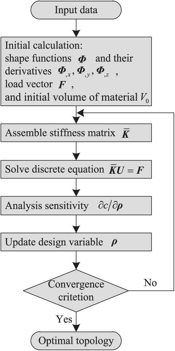
Figure 1: Topology optimization procedure
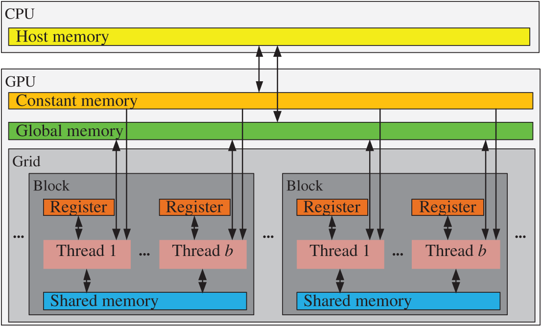
Figure 2: Hierarchy of CUDA thread and memory
4.2 The Reduction Summation Method
In the GPU parallel algorithm, it is necessary to calculate a summation of data for all threads in a thread block. To overcome the problem that using a single thread accumulator would lead to poor performance on a GPU, we adopted a parallel reduction summation strategy in this study. As shown in Fig. 3, b/2 threads (e.g., thread 1–b/2) of all threads executed the pairwise summation during the first step. Analogously, each step of this pairwise summation divided the number of partial sums by half. Ultimately, the sum b was obtained after log2b steps. It was obvious that the number of threads b should be a power of 2.
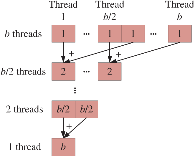
Figure 3: The reduction summation method
As shown in Fig. 4, the same memory location might have had conflicting updates when no less than two threads attempted to access the same memory unit (e.g., units with red color) concurrently. This is an example of the racing of CUDA threads, which could lead to an uncertain outcome. For example, parallelizing the Gauss point-wise approach for the assembly of the stiffness matrix might lead to an uncertain outcome. These race conditions can be avoided with proper algorithms that make a thread write data only to the corresponding memory unit. In addition, atomic operations can avert race conditions by making all updates serialization. In a massively parallel system, however, thousands of threads may be working simultaneously, which can hamper performance. Therefore, atomic operations are suitable only for processing a small number of parallel threads.
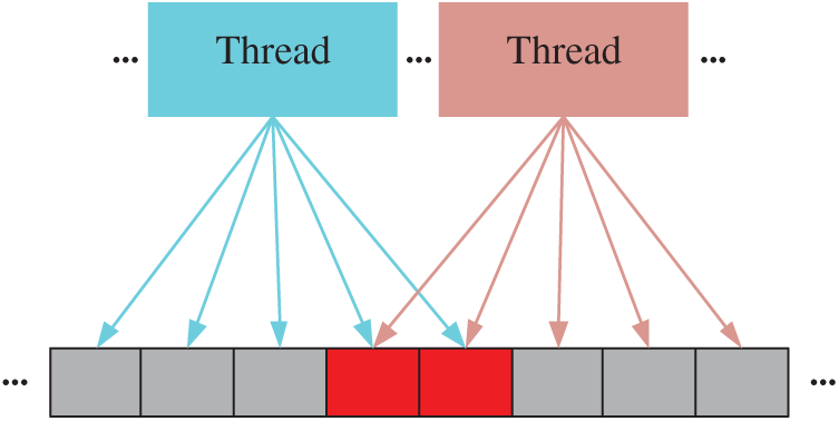
Figure 4: The race conditions
5.1 Assembling Stiffness Matrix
The stiffness matrix
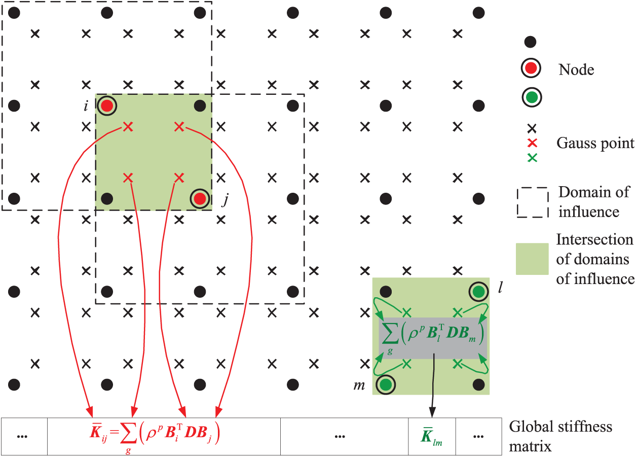
Figure 5: The Gauss point-wise and node pair-wise method for assembling stiffness matrix
The amenability to parallelism of the node pair-wise method is well suited for the GPU parallel computation. As shown in Fig. 6, the GPU parallel algorithm of the node pair-wise method had two levels of parallelism. A thread block handled a node pair related to a specific submatrix, and each thread in a thread block was assigned to a Gauss point of the shared domains of influence of the node pair. When all threads of a thread block completed the calculation, the corresponding 3 × 3 subblock was obtained by the reduction summation method. Note that the number of threads in a thread block should be a power of 2. Finally, the first thread in each thread block wrote the submatrix to the corresponding location in the global memory.
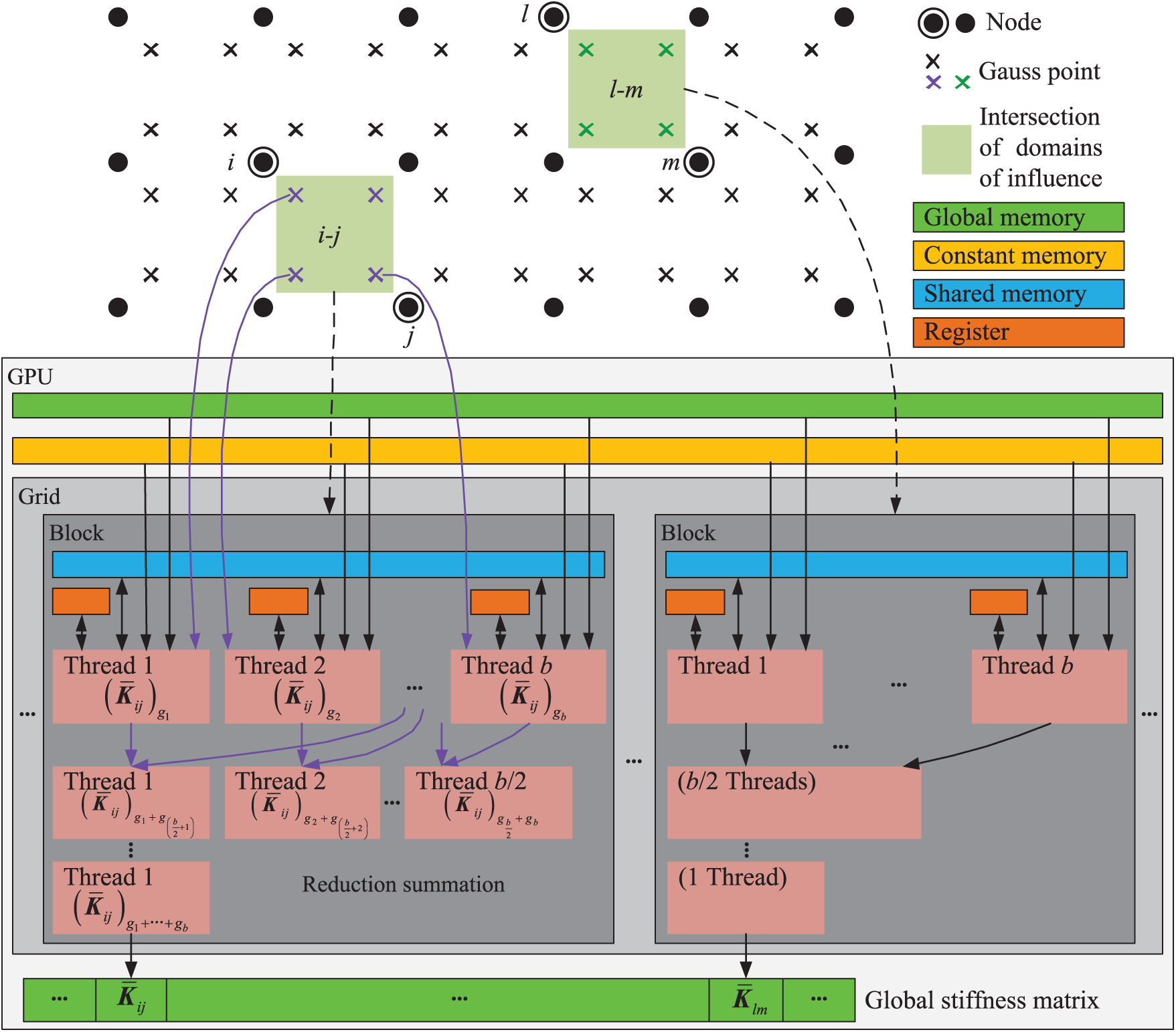
Figure 6: The GPU parallel algorithm for assembling stiffness matrix
5.2 Solving Discrete Equations
In the process of topology optimization, the discrete equations formed by the EFG method need to be solved repeatedly to obtain the structural response. For large-scale problems, in addition to the huge computation time, the use of the direct method is expensive in terms of the storage requirement, resulting from the large number of zeroes that mostly become nonzero values during the factorization process. Therefore, the iterative method usually is employed in the EFG method. The linear equations in topology optimization, however, are extremely ill-conditioned because of the highly heterogeneous material distributions. To improve on the rate of convergence, a preconditioning technique is necessary. In this study, we used the PCG method with the Jacobi preconditioner

The convergence error Tol in the PCG method had a remarkable effect on the solving of linear equations. We obtained more accurate results of linear equations with a stricter error value. Nevertheless, the stricter the convergence error value was, the more PCG iterations at each optimization iteration led to an increase in computing time. In contrast, the topology optimization often is used as a preprocessing stage to find the optimal layout of the material that fulfills the design requirements, and the resulting topology then can be used as the initial guess for further detailed design. If there is a slight change in the density value, the resulting input to the detailed design will not change significantly. Therefore, if we used the PCG method with a loose error to solve the equations, and it had no effect on the topological results, then the time to solve the linear equations could be reduced significantly.
As shown in Fig. 7, the sensitivity of the objective function to the design variable
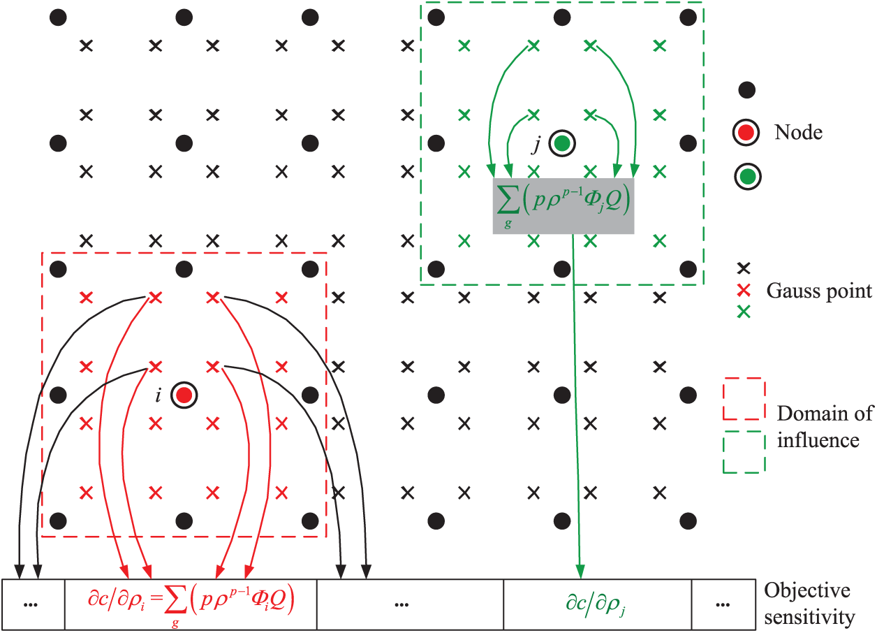
Figure 7: The Gauss point-wise and node-wise method for analyzing sensitivity
We proposed a node-wise method to eliminate the race conditions in the calculation of the objective sensitivity herein. By substituting Eq. (25) into Eq. (23), the sensitivity calculation formula of the objective function can be expressed as follows:
According to the Eq. (26), the computation of the objective sensitivity for each node is split in two steps. In the first step, we calculated the Q values for each Gauss point and stored them for the calculation of the objective sensitivity in the next stage. The required storage of all Q values was small, so storing them temporarily was not an issue. In the second step, we computed the objective sensitivity value corresponding to each node. For node j, the objective sensitivity value
In the first step, we calculated the Q values for all influenced node pairs of every Gauss point, as described in Eq. (27). The two levels of parallelism were as follows: the major over the Gauss points and the minor over the influenced node pairs. This is shown schematically in Fig. 8. We assigned a Gauss point to each thread block (thread number was a power of 2) and each thread handled one influenced node pair at a time. Because each Gauss point corresponded to one thread block, all Q values in the Gauss points were stored in the respective global memory unit.
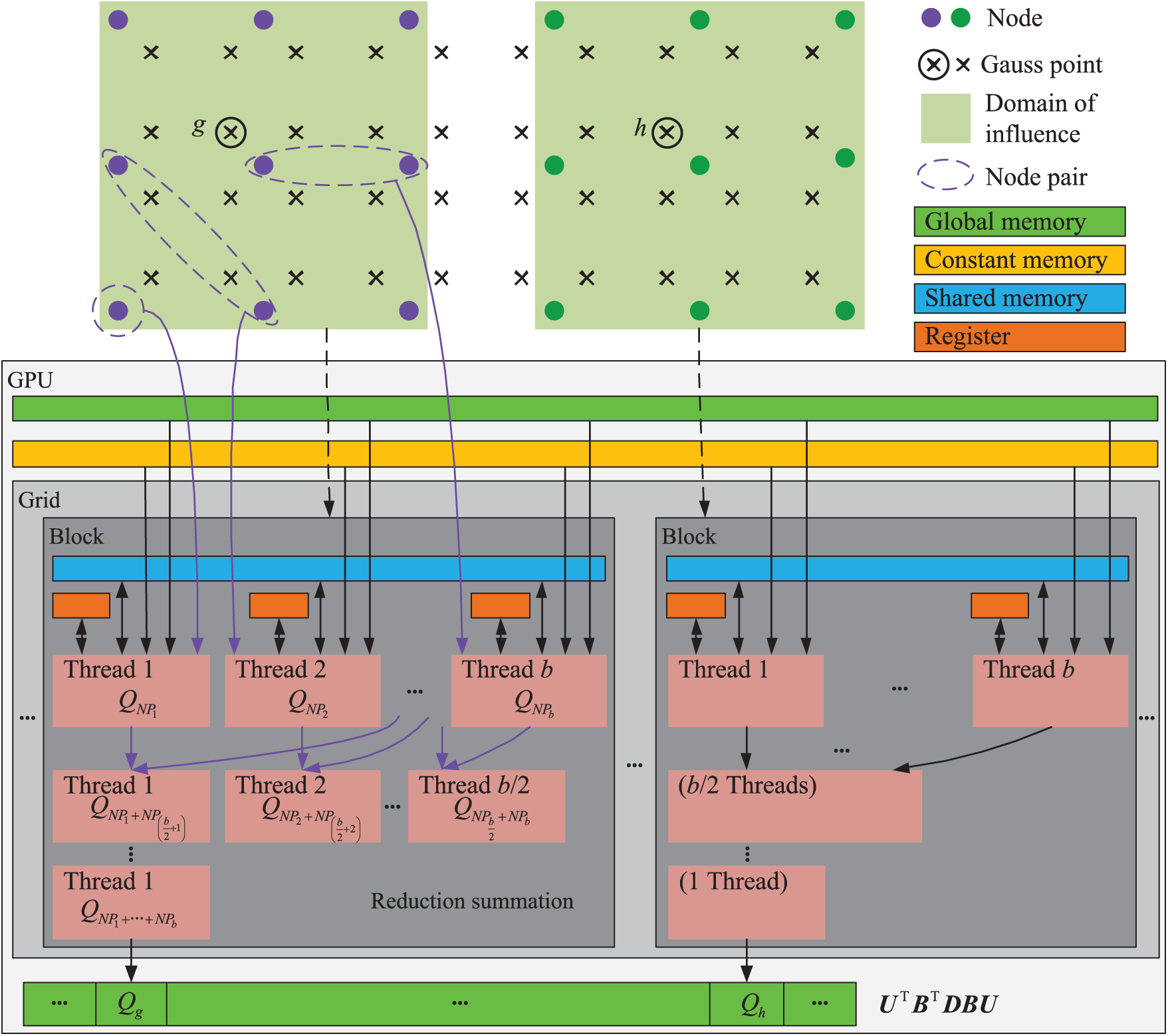
Figure 8: The GPU parallel algorithm for computing the Q values
The GPU parallel algorithm for the calculation of the final value of the objective sensitivity is shown in Fig. 9. We adopted the mode of parallelization similar to the aforementioned parallel strategy, in which each thread block (the number of threads in a thread block should be a power of 2) processed one node at a time and each influenced Gauss point was assigned to one thread. After all influenced Gauss points were processed, the objective sensitivity values of threads of the block were summed according to a reduction summation into the corresponding memory. Because each objective sensitivity value had its own memory unit in the global memory, they were not conflicted in this stage.
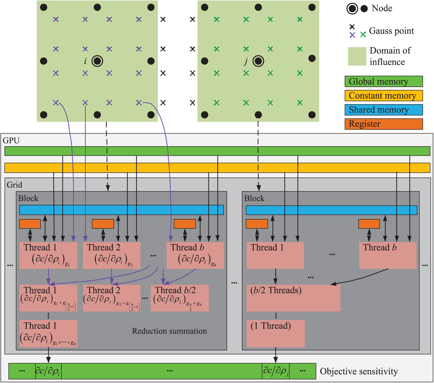
Figure 9: The GPU parallel algorithm for computing the final value of the objective sensitivity
We split the update of the design variable for each node in three stages: calculating the relative density parameter of nodes, the relative density of Gauss points, and the volume of material. Because each design variable was updated independent of the updating of the other design variables according to Eq. (21), the first stage had good parallelism. The GPU parallel strategy of the first stage is illustrated as Fig. 10. To adapt to the hierarchy of CUDA architecture, we organized all nodes in a number of node groups. Each thread block processed a node group, and each thread in the thread block handled a node in the group. After all nodes were processed, the design variable value related to each thread was stored in the corresponding storage unit.

Figure 10: The GPU parallel strategy for calculating the relative density parameter of nodes
The second stage had two levels of parallelism: the major over the Gauss points and the minor over the influenced nodes. As shown in Fig. 11, each Gauss point was assigned to a thread block and each thread handled one affected node. Finally, the reduction sum of values of all threads in each thread block gave the relative density of each Gauss point. Obviously, this stage did not have any race conditions.
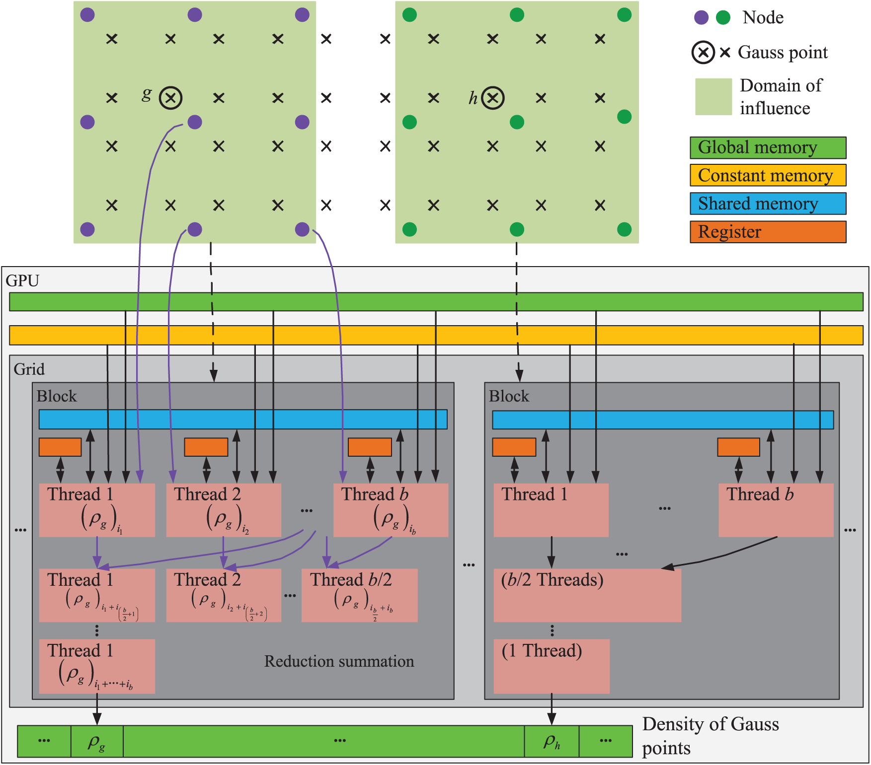
Figure 11: The GPU parallel strategy for calculating the relative density of Gauss points
We adopted the mode of parallelization similar to the parallelization of the first stage in the third stage, as illustrated in Fig. 12. Each thread block dealt with a Gauss point group and each Gauss point was assigned to a thread. Because the number of Gauss point groups was much smaller than the number of Gauss points, we used the atomic operations to avoid the race conditions when the first thread in each thread block wrote the reduction summation to the global memory.
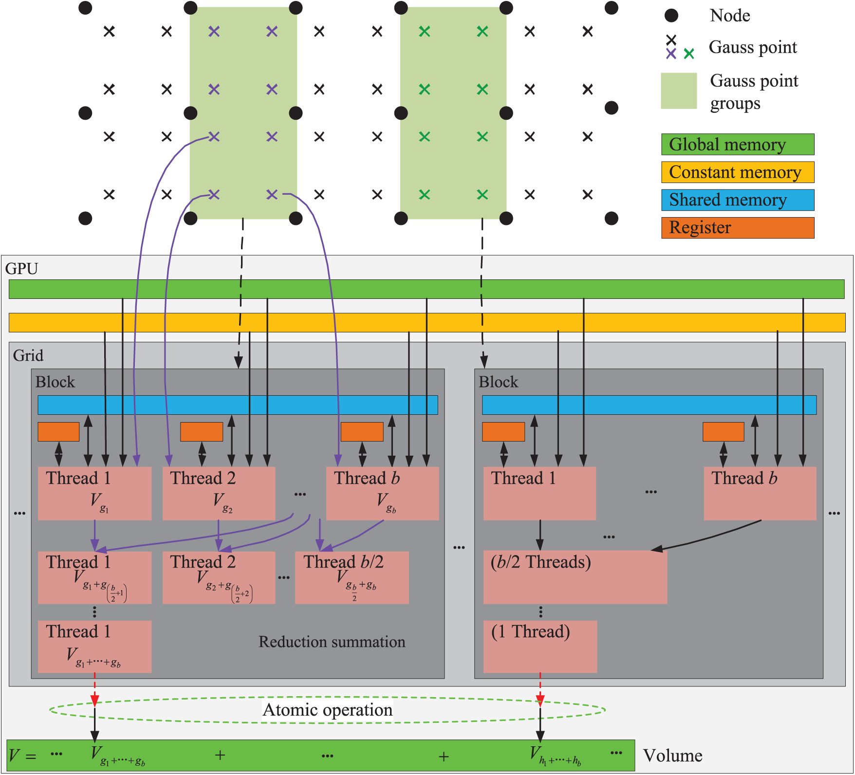
Figure 12: The GPU parallel strategy for calculating the volume of material
The GPU parallel flowchart of topology optimization using the EFG method is shown in Fig. 13. The initial calculation to be executed just once in the flowchart was performed on CPU. The main steps that had to be repeated in the topology optimization process, namely, assembling the stiffness matrix, solving the discrete equation, analyzing sensitivity, and updating the design variables, were parallelized on the GPU to reduce the computation time.
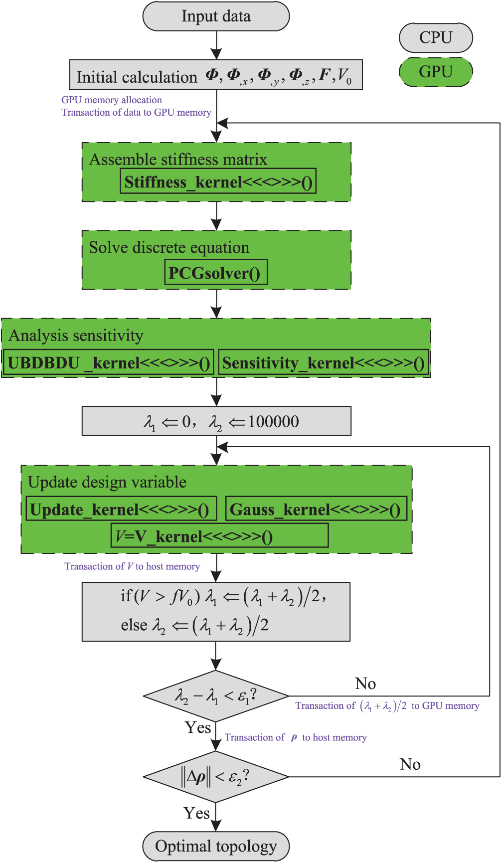
Figure 13: The GPU parallel flowchart of topology optimization using the EFG method
6 Numerical Experiments and Discussions
We evaluated the performance of the proposed GPU parallel algorithm of topology optimization using three numerical examples: the cantilever beam, the quarter annulus, and the cub. The design domain was discretized with a set of meshless field nodes, and a number of virtual background cells were used only for the numerical integration. We used the 2 × 2×2 Gauss quadrature rule for each virtual background cell. The Young's modulus for full-solid region was
(1) Example I: Cantilever Beam
Fig. 14 displays the design domain of a 3D cantilever beam structure. The model size was 100 mm × 50 mm × 4 mm. The left face of the domain was fixed. We applied a vertically downward force
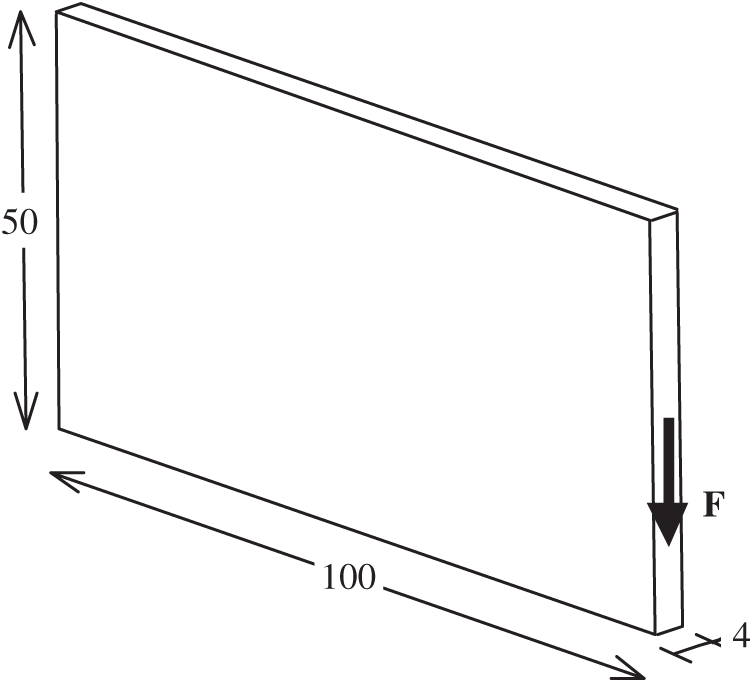
Figure 14: Design domain of the cantilever beam
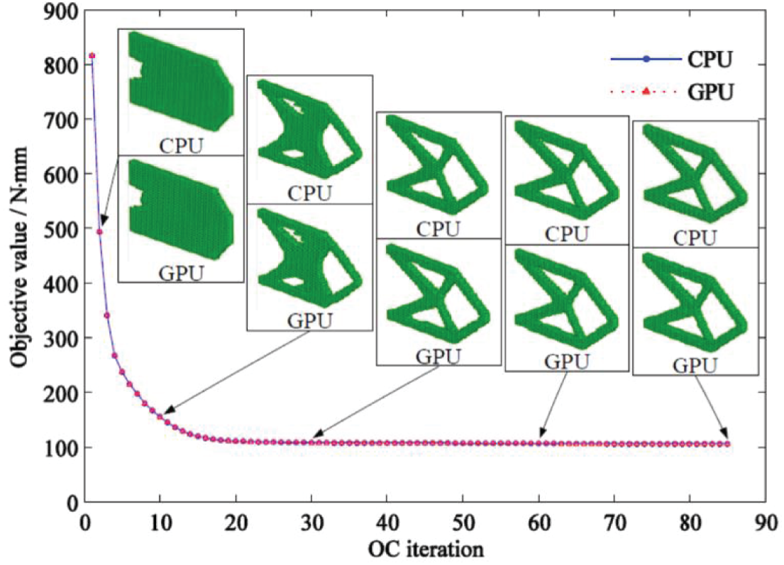
Figure 15: Iteration history and staged results of the cantilever beam topology optimization with CPU and GPU program
(2) Example II: Quarter Annulus
Fig. 16 displays the design domain of a 3D quarter annulus structure and the model size (Unit: mm). The bottom end of the domain was fixed. As shown in the Fig. 16, a horizontal force toward the left was
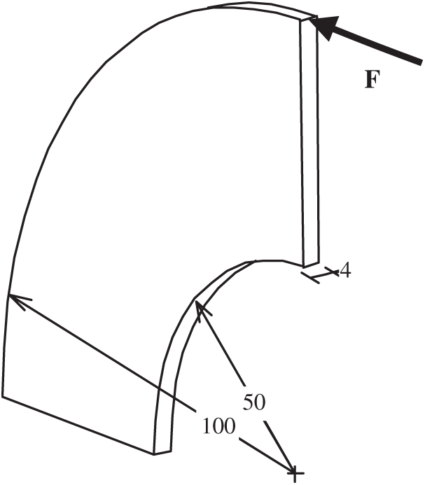
Figure 16: Design domain of the quarter annulus
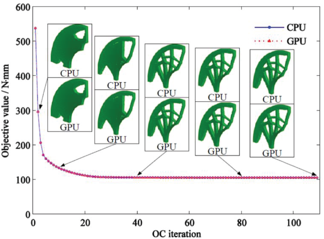
Figure 17: Iteration history and staged results of the quarter annulus topology optimization with CPU and GPU program
(3) Example III: Cube
Fig. 18 displays the design domain of a cub structure. The edge length of the cub was 200 mm. The model was fixed at the gray zones of its lower face, which indicated that the displacements at these surfaces were fixed. We applied a concentrated force
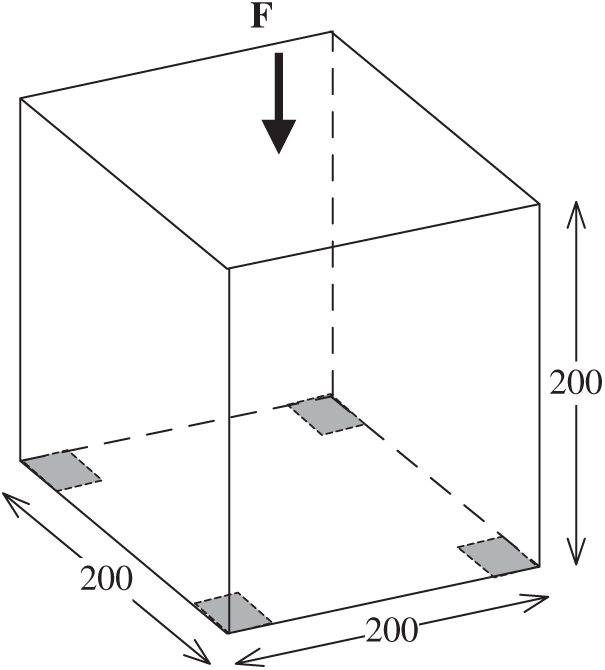
Figure 18: Design domain of the cube
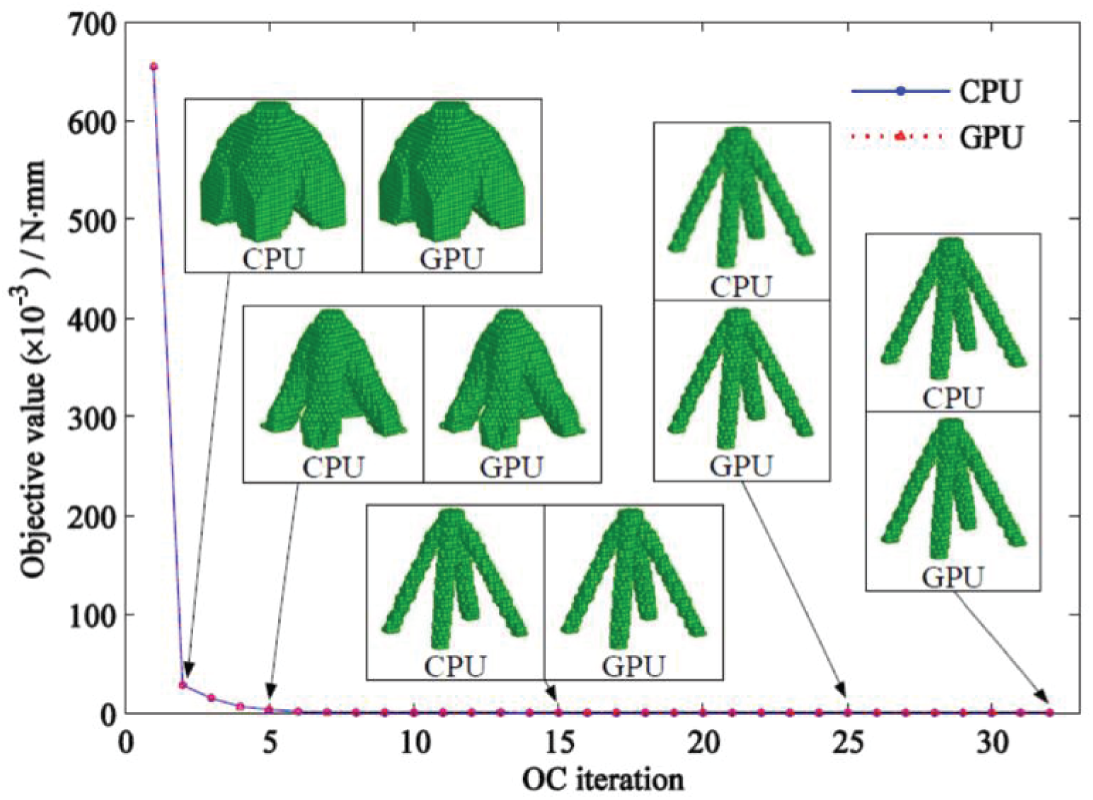
Figure 19: Iteration history and staged results of the cube topology optimization with the CPU and GPU programs
Figs. 15, 17, and 19 show that the staged results and iteration history of topology optimization obtained by using the GPU program proposed in this study are completely consistent with that of the CPU program. This finding further verified the feasibility of the proposed GPU acceleration algorithm and strategy.
6.2 Analysis of Speedup Characteristic
(1) The thread block size
Fig. 20 shows the relationship between the thread block size and the speedup ratio in different stages of three examples.
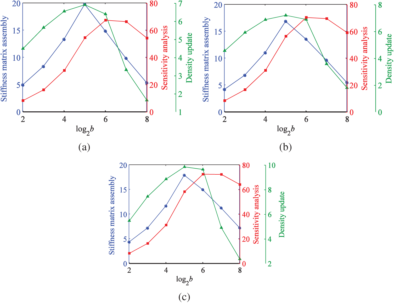
Figure 20: Speedup ratios under different thread block size. (a) Example I (b) Example II (c) Example III
Fig. 20 shows that the speedup ratios increase first and then decrease with the increase of the thread block size. In the GPU algorithm, a greater thread block size was not necessarily better. Under the calculation conditions in this study, the best choice of the thread block size was 32 for the stiffness matrix assembly and density update, and 64 for the sensitivity analysis. This finding also indicated that the GPU algorithm proposed in this study effectively reduced the thread block size, to reduce the occupation of computer resources.
(2) The computing time for different stages
When the PCG error was defined as 1e-5 and the thread block sizes with the best values were chosen, the total computational time for all OC iterations was as given in Tab. 1.

Tab. 1 shows that the assembling stiffness matrix, solving equation, and sensitivity analysis took up most of the time for CPU serial program. Therefore, the computing efficiency of topology optimization was effectively improved by accelerating these three parts using GPU. In addition, although the updating density was not time-consuming, it also had to be computed on GPU to avoid the repeated transmission of large amounts of data between the CPU and GPU. Meanwhile, although the structures of the three numerical examples were different, the speedup ratio of equation solving and overall optimization calculation increased with the increase in the number of DOFs, as shown in Tab. 1, which demonstrated the high efficiency of the proposed GPU parallel approach.
(3) The number of DOFs
When the PCG error was defined as 1e-5 and the thread block sizes with the best values were chosen, the total computing times under different DOFs for Example I were as given in Tab. 2. Global speedup ratios under different DOFs of Example I are shown in Fig. 21. Because of the limitation of computer resources, the maximum total number of DOFs only reached 110,880.

Fig. 21 shows that the speedup ratios will increase with the increase of the DOFs for the same model example before the model scale exceeds the maximum parallel capability of GPU. The GPU was suitable for solving computation-intensive problems; however, the increase of the speedup ratio decreased gradually. This was caused by the limited computing resources of GPU.
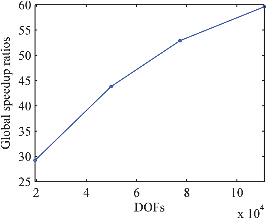
Figure 21: Global speedup ratios under different DOFs of Example I
Simultaneously, because of the use of the interacting node pair method during the stiffness matrix assembly and node-wise method during the sensitivity analysis, the speedup ratios were close to 20 and 70, respectively. Compared with the traditional Gauss point-wise method, their computational efficiency greatly improved. This meant that the use of interacting node pair and node-wise method not only improved the parallelism performance of the GPU, but also effectively avoided the race condition that occurred in the thread-block stored procedures.
In general, the convergence error in the PCG method had a remarkable effect on the solution of discrete equations. The more accurate results of discrete equations could be obtained with more strict error value. Nevertheless, the stricter the error value is, the greater the number of PCG iterations at each optimization iteration leading to increased time. The effect of the convergence error in the PCG method on the topology results and the GPU computing time is shown in Fig. 22.
Fig. 22 shows that when the PCG error value varied from 1e-8 to 1e-1, the final optimal results were basically unchanged, and the number of iterations was about the same. With the relaxation of the error value, the time to solve the equation and the overall optimization time decreased rapidly at first and then increased at the later stage. The increase of the total time was accompanied by an increase of the number of iterations. This meant that the PCG error value could not be relaxed too much, and the recommended error was between 1e-4 and 1e-2.
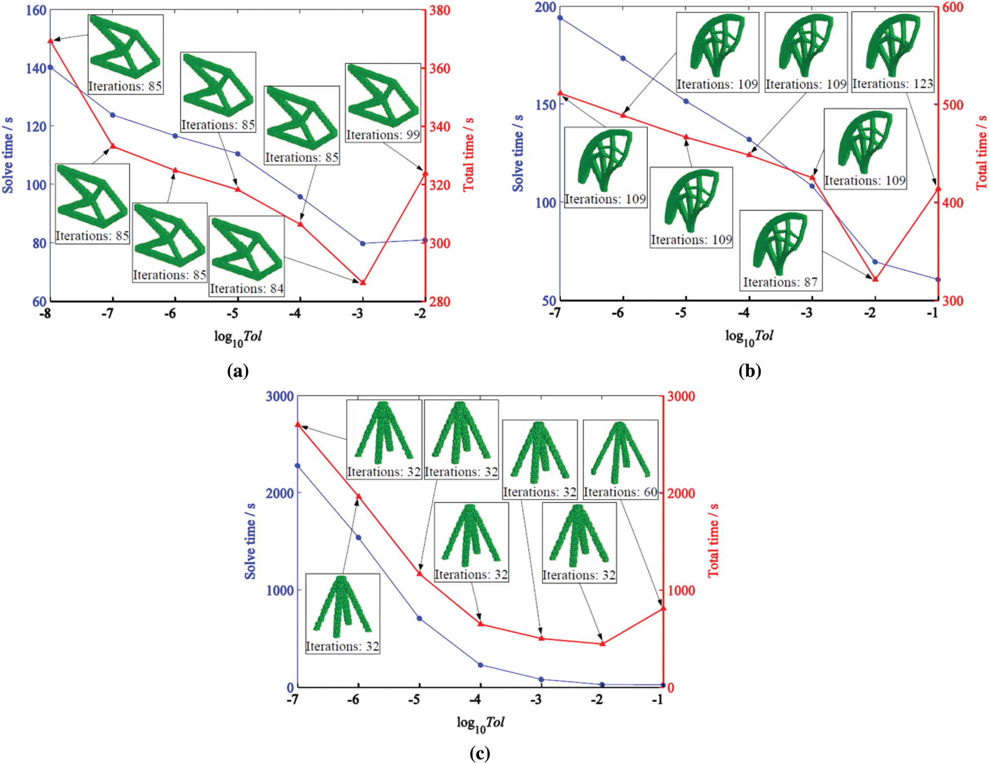
Figure 22: GPU computing performance under different PCG error values. (a) Example I (b) Example II (c) Example III
To improve computational efficiency, we presented a novel GPU acceleration approach for 3D structural topology optimization problems using the EFG method. We developed GPU parallel algorithms of assembling stiffness matrix, solving discrete equation, analyzing sensitivity, and updating design variables. The following conclusions can be drawn from the example analysis:
1. The final optimal structures obtained by the proposed GPU acceleration approach were in good agreement with the CPU results. Thus, the presented approach in this study was feasible. Meanwhile the boundary profiles were clear even without the filtering technique of sensitivity, and there were no checkerboard and other unstable phenomena.
2. Compared with the conventional CPU serial approach, the proposed GPU acceleration approach greatly improved the computational efficiency of 3D structural topology optimization using the EFG method. The maximum of the global speedup ratio of the whole topology optimization process in the examples reached up to 67.8, and the acceleration ratio also increased as the number of DOFs increased. In addition, the thread block size had a significant effect on the computational efficiency. For 3D topology optimization problems, the recommended value of the thread block size was 32 for the stiffness matrix assembly and density update, and 64 for the sensitivity analysis.
3. We used the interacting node pair method during the stiffness matrix assembly and the node-wise method during the sensitivity analysis to effectively improve the parallelism performance of the GPU, and we avoided the race conditions that can occur in thread-block stored procedures.
4. The results showed that the convergence error of the PCG solver used to solve discrete equation at each OC iteration could be properly loosened without qualitatively affecting the resulting topology and leading to a considerable reduction in the solution time of the discrete equation. The overall computing time may have increased as a result of the added OC iterations when loosening the PCG convergence error. Therefore, it is essential to use the appropriate PCG error for topology optimization problems based on the EFG method. The reasonable range of PCG convergence error was between 1e-4 and 1e-2.
Acknowledgement: The support from the National Natural Science Foundation of China (Nos. 51875493, 51975503, 11802261) is appreciated.
Funding Statement: This work is supported by the National Natural Science Foundation of China (Nos. 51875493, 51975503, 11802261). The financial support to the first author is gratefully acknowledged.
Conflicts of Interest: The authors declare that they have no conflicts of interest to report regarding the present study.
1. Deaton, J. D., Grandhi, R. V. (2014). A survey of structural and multidisciplinary continuum topology optimization: Post 2000. Structural and Multidisciplinary Optimization, 49(1), 1–38. DOI 10.1007/s00158-013-0956-z. [Google Scholar] [CrossRef]
2. Zhu, B., Zhang, X., Zhang, H., Liang, J., Zang, H. et al. (2020). Design of compliant mechanisms using continuum topology optimization: A review. Mechanism and Machine Theory, 143, 103622. DOI 10.1016/j.mechmachtheory.2019.103622. [Google Scholar] [CrossRef]
3. Dbouk, T. (2017). A review about the engineering design of optimal heat transfer systems using topology optimization. Applied Thermal Engineering, 112, 841–854. DOI 10.1016/j.applthermaleng.2016.10.134. [Google Scholar] [CrossRef]
4. Xia, L., Breitkopf, P. (2017). Recent advances on topology optimization of multiscale nonlinear structures. Archives of Computational Methods in Engineering, 24, 227–249. DOI 10.1007/s11831-016-9170-7. [Google Scholar] [CrossRef]
5. Liu, J., Gaynor, A. T., Chen, S., Kang, Z., Suresh, K. et al. (2018). Current and future trends in topology optimization for additive manufacturing. Structural and Multidisciplinary Optimization, 57, 2457–2483. DOI 10.1007/s00158-018-1994-3. [Google Scholar] [CrossRef]
6. Sigmund, O., Petersson, J. (1998). Numerical instabilities in topology optimization: A survey on procedures dealing with checker-boards, mesh-dependencies and local minima. Structural Optimization, 16, 68–75. DOI 10.1007/BF01214002. [Google Scholar] [CrossRef]
7. Belytschko, T., Moës, N., Usui, S., Parimi, C. (2001). Arbitrary discontinuities in finite elements. International Journal for Numerical Methods in Engineering, 50, 993–1013. DOI 10.1002/(ISSN)1097-0207. [Google Scholar] [CrossRef]
8. Belytschko, T., Krongauz, Y., Organ, D., Fleming, M., Krysl, P. (1996). Meshless methods: An overview and recent developments. Computer Methods in Applied Mechanics and Engineering, 139(1–4), 3–47. DOI 10.1016/S0045-7825(96)01078-X. [Google Scholar] [CrossRef]
9. Cho, S., Kwak, J. (2006). Topology design optimization of geometrically non-linear structures using meshfree method. Computer Methods in Applied Mechanics and Engineering, 195(44–47), 5909–5925. DOI 10.1016/j.cma.2005.08.015. [Google Scholar] [CrossRef]
10. Lin, J., Guan, Y., Zhao, G., Naceur, H., Lu, P. (2017). Topology optimization of plane structures using smoothed particle hydrodynamics method. International Journal for Numerical Methods in Engineering, 110(8), 726–744. DOI 10.1002/nme.5427. [Google Scholar] [CrossRef]
11. Belytschko, T., Lu, Y. Y., Gu, L. (2012). Element-free galerkin methods. International Journal for Numerical Methods in Engineering, 37, 229–256. DOI 10.1002/nme.1620370205. [Google Scholar] [CrossRef]
12. Gong, S. G., Chen, M., Zhang, J. P., He, R. (2012). Study on modal topology optimization method of continuum structure based on EFG method. International Journal of Computational Methods, 9(1), 1240005. DOI 10.1142/S0219876212400051. [Google Scholar] [CrossRef]
13. He, Q. Z., Kang, Z., Wang, Y. Q. (2014). A topology optimization method for geometrically nonlinear structures with meshless analysis and independent density field interpolation. Computational Mechanics, 54, 624–629. DOI 10.1007/s00466-014-1011-7. [Google Scholar] [CrossRef]
14. Shobeiri, V. (2016). Topology optimization using bi-directional evolutionary structural optimization based on the element-free galerkin method. Optimization and Engineering, 48(3), 380–396. DOI 10.1080/0305215X.2015.1012076. [Google Scholar] [CrossRef]
15. Shobeiri, V. (2015). The topology optimization design for cracked structures. Engineering Analysis with Boundary Elements, 58, 26–38. DOI 10.1016/j.enganabound.2015.03.002. [Google Scholar] [CrossRef]
16. Zhang, Y. Q., Ge, W. J., Zhang, Y. H., Zhao, Z. F., Zhang, J. W. (2018). Topology optimization of hyperelastic structure based on a directly coupled finite element and element-free galerkin method. Advances in Engineering Software, 123, 25–37. DOI 10.1016/j.advengsoft.2018.05.006. [Google Scholar] [CrossRef]
17. Khan, W., Islam, S., Ullah, B. (2019). Structural optimization based on meshless element free galerkin and level set methods. Computer Methods in Applied Mechanics and Engineering, 344, 144–163. DOI 10.1016/j.cma.2018.09.024. [Google Scholar] [CrossRef]
18. Zhang, J. P., Wang, S. S., Zhou, G. Q., Gong, S. G., Yin, S. H. (2020). Topology optimization of thermal structure for isotropic and anisotropic materials using the element free galerkin method. Engineering Optimization, 52(7), 1097–1118. DOI 10.1080/0305215X.2019.1636979. [Google Scholar] [CrossRef]
19. Metsis, P., Papadrakakis, M. (2012). Overlapping and non-overlapping domain decomposition methods for large-scale meshless EFG simulations. Computer Methods in Applied Mechanics and Engineering, 229, 128–141. DOI 10.1016/j.cma.2012.03.012. [Google Scholar] [CrossRef]
20. Trask, N., Maxey, M., Kim, K., Perego, M., Parks, M. L. et al. (2015). A scalable consistent second-order SPH solver for unsteady low reynolds number flows. Computer Methods in Applied Mechanics and Engineering, 289, 155–178. DOI 10.1016/j.cma.2014.12.027. [Google Scholar] [CrossRef]
21. Singh, R., Singh, K. M. (2018). On preconditioned BiCGSTAB solver for MLPG method applied to heat conduction in 3D complex geometry. Engineering Analysis with Boundary Elements, 93, 83–93. DOI 10.1080/10407782.2017.1400335. [Google Scholar] [CrossRef]
22. Danielson, K. T., Hao, S., Liu, W. K., Uras, R. A., Li, S. (2000). Parallel computation of meshless methods for explicit dynamic analysis. International Journal for Numerical Methods in Engineering, 47, 1323–1341. DOI 10.1002/(SICI)1097-0207(20000310)47:7<1323::AID-NME827>3.0.CO;2-0. [Google Scholar] [CrossRef]
23. Singh, I. V. (2004). Parallel implementation of the EFG method for heat transfer and fluid flow problems. Computational Mechanics, 34(6), 453–463. DOI 10.1007/s00466-004-0590-0. [Google Scholar] [CrossRef]
24. Cecka, C., Lew, A. J., Darve, E. (2011). Assembly of finite element methods on graphics processors. International Journal for Numerical Methods in Engineering, 85(5), 640–669. DOI 10.1002/nme.2989. [Google Scholar] [CrossRef]
25. Wang, H., Zeng, Y., Li, E., Huang, G. X., Gao, G. Q. et al. (2016). “Seen is solution” a CAD/CAE integrated parallel reanalysis design system. Computer Methods in Applied Mechanics and Engineering, 299, 187–214. DOI 10.1016/j.cma.2015.10.022. [Google Scholar] [CrossRef]
26. Liu, R. K. S., Wu, C. T., Kao, N. S. C., Sheu, T. W. H. (2019). An improved mixed lagrangian–Eulerian (IMLE) method for modelling incompressible navier–Stokes flows with CUDA programming on multi-GPUs. Computer & Fluids, 184, 99–106. DOI 10.1016/j.compfluid.2019.03.024. [Google Scholar] [CrossRef]
27. Torky, A. A., Rashed, Y. F. (2017). GPU acceleration of the boundary element method for shear-deformable bending of plates. Engineering Analysis with Boundary Elements, 74, 34–48. DOI 10.1016/j.enganabound.2016.10.006. [Google Scholar] [CrossRef]
28. Karatarakis, A., Metsis, P., Papadrakakis, M. (2013). GPU-Acceleration of stiffness matrix calculation and efficient initialization of EFG meshless methods. Computer Methods in Applied Mechanics and Engineering, 258, 63–80. DOI 10.1016/j.cma.2013.02.011. [Google Scholar] [CrossRef]
29. Dong, Y., Grabe, J. (2018). Large scale parallelisation of the material point method with multiple GPUs. Computers and Geotechnics, 101, 149–158. DOI 10.1016/j.compgeo.2018.04.001. [Google Scholar] [CrossRef]
30. Frissane, H., Taddei, L., Lebaal, N., Roth, S. (2019). 3D smooth particle hydrodynamics modeling for high velocity penetrating impact using GPU: Application to a blunt projectile penetrating thin steel plates. Computer Methods in Applied Mechanics and Engineering, 357, 112590. DOI 10.1016/j.cma.2019.112590. [Google Scholar] [CrossRef]
31. Chen, X., Wan, D. (2019). GPU accelerated MPS method for large-scale 3-D violent free surface flows. Ocean Engineering, 171, 677–694. DOI 10.1016/j.oceaneng.2018.11.009. [Google Scholar] [CrossRef]
32. Afrasiabi, M., Meier, L., Röthlin, M., Klippel, H., Wegener, K. (2020). GPU-Accelerated meshfree simulations for parameter identification of a friction model in metal machining. International Journal of Mechanical Sciences, 176, 105571. DOI 10.1016/j.ijmecsci.2020.105571. [Google Scholar] [CrossRef]
33. Challis, V. J., Roberts, A. P., Grotowski, J. F. (2014). High resolution topology optimization using graphics processing units (GPUs). Structural and Multidisciplinary Optimization, 49(2), 315–325. DOI 10.1007/s00158-013-0980-z. [Google Scholar] [CrossRef]
34. Martínez-Frutos, J., Herrero-Peréz, D. (2016). Large-scale robust topology optimization using multi-GPU systems. Computer Methods in Applied Mechanics and Engineering, 311, 393–414. DOI 10.1016/j.cma.2016.08.016. [Google Scholar] [CrossRef]
35. Martinez-Frutos, J., Herrero-Perez, D. (2017). GPU acceleration for evolutionary topology optimization of continuum structures using isosurfaces. Computers & Structures, 182, 119–136. DOI 10.1016/j.compstruc.2016.10.018. [Google Scholar] [CrossRef]
36. Martinez-Frutos, J., Martinez-Castejon, P. J., Herrero-Perez, D. (2017). Efficient topology optimization using GPU computing with multilevel granularity. Advances in Engineering Software, 106, 47–62. DOI 10.1016/j.advengsoft.2017.01.009. [Google Scholar] [CrossRef]
37. Ramirez-Gil, F., Nelli-Silva, E., Montealegre-Rubio, W. (2016). Topology optimization design of 3D electrothermomechanical actuators by using GPU as a co-processor. Computer Methods in Applied Mechanics and Engineering, 302, 44–69. DOI 10.1016/j.cma.2015.12.021. [Google Scholar] [CrossRef]
38. Xia, Z., Wang, Y., Wang, Q., Mei, C. (2017). GPU parallel strategy for parameterized LSM-based topology optimization using isogeometric analysis. Structural and Multidisciplinary Optimization, 56(2), 413–434. DOI 10.1007/s00158-017-1672-x. [Google Scholar] [CrossRef]
 | This work is licensed under a Creative Commons Attribution 4.0 International License, which permits unrestricted use, distribution, and reproduction in any medium, provided the original work is properly cited. |