Computer Modeling in Engineering & Sciences

DOI: 10.32604/cmes.2021.015773

ARTICLE

Discontinuous-Galerkin-Based Analysis of Traffic Flow Model Connected with Multi-Agent Traffic Model

Rina Okuyama1, Naoto Mitsume2, Hideki Fujii1 and Hideaki Uchida1,*

1The University of Tokyo, 7-3-1 Hongo, Bunkyo-ku, Tokyo, 113-8656, Japan
2University of Tsukuba, 1-1-1 Tennodai, Tsukuba City, Ibaraki, 305-8577, Japan
*Corresponding Author: Hideaki Uchida. Email: uchida@sys.t.u-tokyo.ac.jp; uchida@see.eng.osaka-u.ac.jp
Received: 12 January 2021; Accepted: 15 April 2021

1  Introduction

As the number of owned automobiles continues to increase year after year, the associated problem of traffic congestion has become a serious societal issue, responsible not only for lost time but also for increased emission of greenhouse gases and other harmful environmental effects. To date, proposals for reducing traffic congestion have called for the construction of bypasses and similar remedies, but the problem will not be solved by simply increasing road space alone. The primary reason for this is that, when the transportation capacity of a given thoroughfare is increased, it receives new users who had previously been using other roads, and this release of latent demand ensures that the congestion state remains unchanged. Moreover—as shown, for example, by the paradox discussed in [1]—situations in which individual drivers pursue their own individual utility do not necessarily coincide with states of optimal traffic flow overall, and there are even cases in which new thoroughfares created to reduce travel times in road networks in fact induce traffic redistributions that ultimately increase travel times.

Initiatives to mitigate these problems have considered not only simply expanding traffic capacity, but also optimizing traffic volumes in wide-area road networks, and traffic-flow simulation has become a focus of interest as a technique for advance characterization of such strategies. Indeed, through effective use of traffic-flow simulation one can reconstruct traffic systems, under a variety of conditions, at a tiny fraction of the cost of experiments using actual roads. Moreover, solving traffic problems requires an understanding of the causes, timing, and location of traffic congestion, as well as insight into how congestion propagates through road networks, and traffic-flow simulations also offer an efficient way to obtain results from this perspective. This situation has spurred the development of a variety of traffic-flow simulators, including ADVENTURE_Mates (Multi-Agent based Traffic and Environment Simulator) [2,3], NETSIM (NETwork SIMulator) [4] SATURN (Simulation and Assignment of Traffic in Urban Road Networks) [5], and SUMO (Simulation of Urban MObility) [6],

In this study, we design a multiscale traffic-flow model in which traffic-flow information is mutually exchanged between microscopic and macroscopic models. The proposition of this model is the first step in future simulations of large-scale road networks considering localized effects such as lane regulation and street parking, which are difficult to express in macroscopic models. The specific models we combine to yield our multiscale model are the generalized force model [7], a type of car-following model, and the Payne–Whitham (PW) model [8,9], a non-equilibrium and fluid-approximated traffic model. Our procedure for combining these constituents yields several advantages for the model and simulations based on it. First, our proposed model can reduce computational costs by avoiding simulations of the entire area using macroscopic models because it enables us to locally use a microscopic model in simulations that utilize microscopic models. Second, our proposed model guarantees the conservation of the number of vehicles at the micro/macro interface, which is not trivial between the continuum expression as the density distribution and the agent-based one. Third, we simulate the macroscopic models using discontinuous Galerkin finite element method (DGFEM) [10–12], which enables us to use an arbitrary polynomial order in each element (road section) and guarantees the conservation of quantities. This is a theoretical extension of the cell transmission method (CTM) [13,14] used in existing studies on multi-scale models. In addition, we adopt a generating/absorbing sponge layer [15], a technique widely used to deal with the inflow/outflow boundary conditions in the numerical analysis of shallow water equations for future applications, to simulate large-scale road networks.

This paper is organized as follows. In this Introduction, we reviewed the fundamentals of traffic-flow models and their societal significance, surveyed prior research, and outlined the research presented here and the objectives of our study. In Section 2, we conducted a survey of conventional researches. In Section 3, we present an outline of our traffic-flow model. In Section 4, we discuss a method for discretizing our macroscopic traffic-flow model. In Section 5, we will describe the methodology of connecting the two models described up to this point, In Section 6, present an example of a simulation using the traffic-flow model of this paper. Finally, In Section 7, we present our conclusions and discuss avenues for future work.

2  Literature Review

Traffic-flow models may be broadly divided into two categories based on granularity: microscopic models, which separately track the motion of all vehicles to yield detailed descriptions of the behaviour of each individual vehicle in a model, and macroscopic models, which consider the vehicle densities in a traffic flow and apply methods of fluid mechanics. Because microscopic traffic-flow models consider the behaviour of individual vehicles, they are capable of producing highly detailed results, but the very nature of these models makes their simulations computationally costly, and enormous computation time is required to recreate traffic flows over wide geographical areas. In contrast, macroscopic traffic-flow models do not attempt to resolve the behaviour of individual vehicles, but rather represent traffic flows in terms of macroscopic quantities—such as traffic volumes, vehicle densities, and space mean velocities—associated with specific points or sections in time and space. These models do not attempt to capture the state of individual vehicles, so their simulation requires relatively little computation time, even for models spanning wide geographical areas.

Because traffic-flow simulations are designed to model traffic systems under a variety of conditions, they must produce detailed results that reflect minor variations in the operating environment. Moreover, it is impossible to measure parameters of individual cars and drivers accurately in actual traffic systems, and thus traffic-flow simulation must be constructed by components incorporating randomness in order to represent parameter distributions. This requires that simulations be performed multiple times, even with identical parameter settings, with different random seeds; consequently, each individual simulation must require only a short period of time to complete if one is to have any hope of testing multiple sets of operating conditions.

In actual traffic flows, certain road segments—such as segments with merge points, sags, or traffic lights—act as bottlenecks from which traffic congestion frequently arises. The challenge of simulating such phenomena has motivated the introduction of multiscale models, which combine a microscopic model for specific subregions with a macroscopic model for all other subregions. Using a microscopic model enables detailed local analysis of segments where traffic congestions or accidents often occur, and combining macroscopic models allows wide peripheral geographical areas to be calculated at a low computational cost.

To date, studies of multiscale traffic-flow models have employed mathematical techniques to connect microscopic and macroscopic models and convert between the two domains. Reference [16] considered a multiscale traffic-flow model consisting of a car-following model [17], which is one of the most popular microscopic traffic-flow models, paired with the LWR model (the Lighthill–Whitham–Richards model [18,19]), which is one of the fundamental microscopic traffic-flow models, and proposed methods for determining boundary conditions and scale transformations. Similarly, Lattanzio et al. [20] discussed a multiscale traffic-flow model combining a car-following model with a different choice of continuous macroscopic model (the Aw–Rascle–Zhang model [21,22]). In [23,24], a macro gray prediction model was established by combining the micro-car-following model and tensor model to predict traffic flow.

The scope of both of these studies was restricted to presenting transformation formulas and mathematical proofs for transferring computational results between microscopic and macroscopic traffic-flow models, and to date the models have not been verified in the way of traffic engineering or applied to practical situation. Moreover, the model of Garavello et al. used an equilibrium traffic model for the macroscopic domain; such models, in which the velocity is uniquely determined by the density, cannot reproduce realistic traffic flows. The model of Lattanzio et al. used a non-equilibrium traffic model, but improvements to the stability of this model were left as a topic for future work. In a related research field, recent efforts have been devoted to the derivation of macroscopic models from kinetic equations (mesoscopic models) [25,26], and this derivation highlights the role of conserved quantities at the microscopic level.

3  Traffic Flow Model

3.1 Multiscale Traffic-Flow Model

In this study, we combine two traffic-flow models, one microscopic and one macroscopic, with the goal of achieving high-precision traffic-flow simulation at low computational cost. In this section, we discuss the key features of each model; our procedure for combining the models is discussed in the following section.

3.2 Generalized Force Model

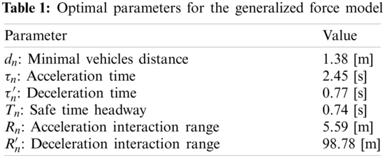
The microscopic model used in this study is the generalized force model (GFM) of Helbing et al. [7].

dvndt=vn(0)−vnτn+fn,n−1(xn,vn;xn−1,vn−1) (1)

fn.n−1=V(sn)−vn(0)τn−ΔvnΘ(Δvn)τ′nexp⁡(−(sn−s(vn))R′n) (2)

s(vn)=dn+Tnvn (3)

V(sn)=V(sn,vn)=vn(0){1−exp⁡(−sn−sn(vn)Rn)} (4)

Tab. 1 lists the optimal parameter values suggested by Helbing et al. [7]. We use these values for all simulations presented in this paper.

3.3 Payne–Whitham Model

A traffic flow comprising the motion of many vehicles may be viewed macroscopically as a continuous fluid. Continuous macroscopic traffic-flow models are models that adopt this point of view, describing vehicle traffic as the motion of a continuous fluid and interpreting coarse-grained fluctuations in traffic density as the propagation of waves through this fluid. These models boast the advantage of modest computational cost even for simulations encompassing large numbers of vehicles but suffer from the drawback that they are essentially incapable of capturing the behavior of individual vehicles. Although there do exist a small number of macroscopic traffic-flow models that distinguish vehicles of different types—such as passenger vehicles, trucks, and buses—even in such cases, all vehicles of a given type are treated as identical indistinguishable elements. Descriptions of this sort are clearly limited in their ability to represent actual real-world traffic flows, which involve vehicles of many different types, operated by drivers of many different driving styles, thereby giving rise to unpredictable traffic flows. Moreover, the data-acquisition capabilities of continuous macroscopic models are limited to two macroscopic quantities, the density and average velocity of vehicles within a finite segment of a road, and are insufficient to yield a complete re-creation of actual realistic traffic flows. The continuum equation, which means the total number of vehicles is conserved, is written as follows: Eq. (5), where ρ is the density of vehicles.

∂ρ∂t+∂ρv∂x=0 (5)

Eq. (5) describes a general macroscopic traffic-flow model. Because the model involves two variables, the density ρ and velocity v, this single equation does not suffice to predict the density and velocity at the next time step; to proceed, we must augment our system by the addition of a second independent equation, and strategies for obtaining this equation may be broadly classified into two categories: equilibrium traffic models (ETMs)—in which the velocity is taken to be a function of the density, and the additional equation is (5), expressing the functional dependence v = v(ρ)—and non-equilibrium traffic models (NETMs), which augment (5) by a separate partial differential equation in which the density and velocity appear as independent variables.

In this context, the term “equilibrium” refers to the fact that, in ETMs, all traffic phenomena arise in accordance with a single equilibrium curve (ρ, v(ρ):ρ) ∈ [0, ρm]; NETMs relax this restriction by adding a new partial differential equation describing the rate of change of the velocity, thus enabling the emergence of non-equilibrium states.

To compensate for this limitation of ETMs—that, by imposing a velocity-density relation, they constrain traffic flows to lie within the equilibrium state curve—higher-order equations approximating the fluid-mechanical law of momentum conservation have been proposed; for example, for the velocity-density relation one might introduce a partial differential equation describing the rate of change of the velocity. In this study, we adopt the PW model, an NETM described by the following equations:

∂ρ∂t+∂∂x(ρv)=0 (6)

∂v∂t+v∂v∂x+1ρ∂p(ρ)∂x=1τ(V(ρ)−v) (7)

In this study, for the equilibrium velocity of the macroscopic traffic-flow model, we use the equation derived by Greenshields et al. [27] based on the results of actual experimental measurements.

4  Discretization Using Discontinuous Galerkin Method with Sponge Layer Model

4.1 Generating/Absorbing Sponge Layer Model

We adopt an generating/absorbing layer model [28,29] to impose the inflow and outflow boundary condition in this study. This model has been widely used for numerical simulation of the shallow water equations. The following equations are solved instead of Eqs. (6) and (7):

∂ρ∂t+∂q∂x=s1in+s1out (8)

∂q∂t+∂∂x(q2ρ+c02ρ)=1τ(ρV(ρ)−q)+s2in+s2out (9)

where sin1 and sin2 are additional terms for inflow boundary condition, and sout1 and sout2 are ones for outflow boundary condition defined as follows:

s1in=χin(ρin−ρ),s2in=χin(qin−q) (10)

s1out=χout(ρout−ρ),s2out=χout(qout−q) (11)

χin(x)=winc0Δt{lin−(x−xL)lin}2(xL≤x≤xL+lin) (12)

χout(x)=woutc0Δt{lout−(xR−x)lout}2(xR−lout≤x≤xR). (13)

Here, ρin and qin are the imposed density and flow rate at the inflow boundary, and ρout and qout are the imposed density and flow rate at the outflow boundary. xL and xR are positions of inflow and outflow boundaries. lin and lout are lengths of layers at inflow and outflow boundaries. win and wout are parameters to adjust the effectiveness of layers. A schematic view of these layers is shown in Fig. 1.

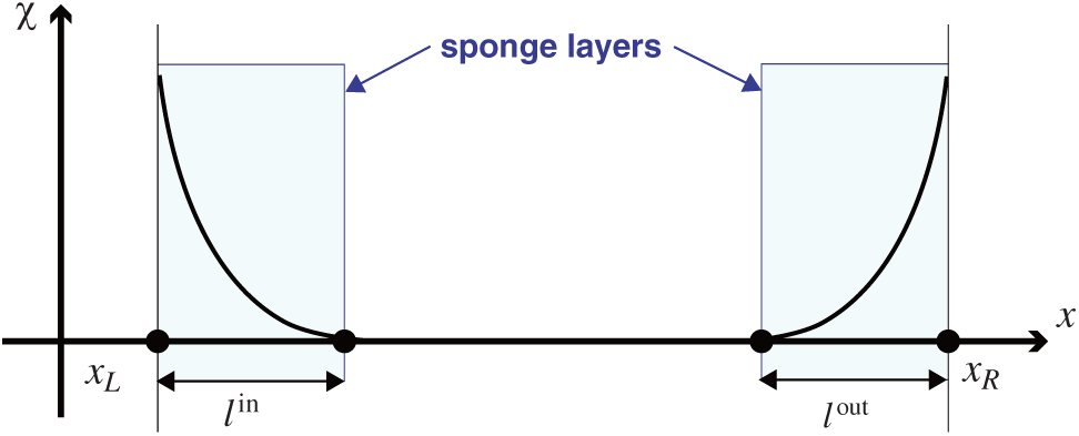
Figure 1: Schematic view of sponge layers and corresponding χ values

4.2 Discontinuous-Galerkin Finite Element Method

The discontinuous Galerkin finite element method (DGFEM) [10], which admits discontinuity of solution between elements as shown in Fig. 2, can be regarded as an extension of both the finite element method and finite volume method. While DGFEM is based on the finite element interpolation with the Lagrange polynomial inside each element, there is the numerical flux at the interface of each element, which is determined by solving the Riemann problem.

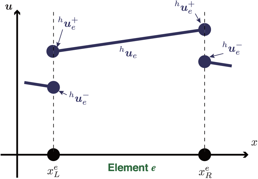
Figure 2: Distribution of u in discontinuous-Galerkin method

The divergence form of Eqs. (8) and (9) can be written as follows:

∂u∂t+∂∂x(f(u))=s(u)u={ρq},f(u)={qq2ρ+c02ρ},s(u)={s1in+s1out1τ(ρV(ρ)−q)+s2in+s2out}. (14)

u is discretized using the corresponding nodal values, ui (i = 1, … ,N), and the shape functions in an element, ψi (i = 1, … ,N), as follows:

hu(x)=∑i=1Nuiψi(x), (15)

where N is the number of nodes in each element. We use N − 1th order Lagrange polynomials defined in normalized space ξ ∈ ( −1, 1),

LiN−1(ξ)=∏j=1,i≠jNξ−ξjξi−ξj(i=1,2,…,N) (16)

as shape functions as follows:

ψi(x)=LiN−1(ξ(x)) (17)

Letting Ωe ∈ (xeL, xeR) be the area of element e, weighted residual equations of Eq. (14) in element e are given as follows:

∫xLexRe∂hue∂tψidx−∫xLexRef(hue)∂ψi∂xdx+[f^(hue+,hue−)ψi]xLexRe=∫xLexRes(hue)ψidx, (18)

where hue+ and hue− are the numerical solution of along the interior and the exterior of element e, respectively, as shown in Fig. 2. f^(hue+,hue−) is the numerical flux. We use the local Lax-Friedrich flux,

f^(hue+,hue−)=12{f(hue+)+f(hue−)−12C(hue+−hue−)} (19)

to determine the numerical flux in this study.

4.3 Time Integration

Substituting Eq. (15) into Eq. (18), following linear equations of element e are derived:

Me_∂Ue_∂t=Re_, (20)

where Ue_ and Re_ are 2 × N martices, and Me_ is N × N matrix defined as follows:

[Me_]ij=∫xLexReψiψjdx,Ue_=[(u1e)T⋮(uNe)T],Re_=[(R1e)T⋮(RNe)T] (21)

Rie=∫xLexRe{f(hue)∂ψi∂x+s(hue)ψi}dx−[f^(hue+,hue−)ψi]xLexRe (22)

Applying the explicit Euler method to Eq. (24), Ue_ in n + 1 step, Ue_n+1, can be computed as follows:

Ue_n+1=Ue_n+ΔtMe_−1Re_. (23)

5  Connecting the PW Model to the GFM

In this section, we use a working example to illustrate our procedure for connecting the PW model to the GFM and converting between the two models. We begin by converting computational results obtained for the PW model into data that may be processed by the GFM. This involves computing the number of vehicles passing through the PW model flow outlet on each timestep. After using DGFEM to analyze the PW model, the number of vehicles passing through the flow outlet may be computed via either of two methods. The first option is to integrate the flow outlet sponge-layer coefficient sρout with respect to time. Using Euler’s method to discretize the time axis with a fixed timestep Δ{t}, the number Cn of outflowing vehicles on the nth timestep takes the following form:

Cn=∫nΔt(n+1)Δt∫xLxRsρoutdxdt≃∫xLxRsρoutdxΔt (24)

However, in this approach, it is difficult to determine uniquely the positions and velocities of outflowing vehicles. The alternative option is to place the connecting region at a point xcon lying upstream from the sponge layer. The concept of the approach is shown in Fig. 3. The time integral of the traffic volume qcon at that point then determines Cn. The “con” superscript labels quantities associated with the connecting region.

Cn=∫nΔt(n+1)Δtqcondt≃qconΔt. (25)

Using this method, the density qcon at the location of the connecting region may be used to determine the velocity vcon at that point according to the following:

vcon=qconρcon (26)

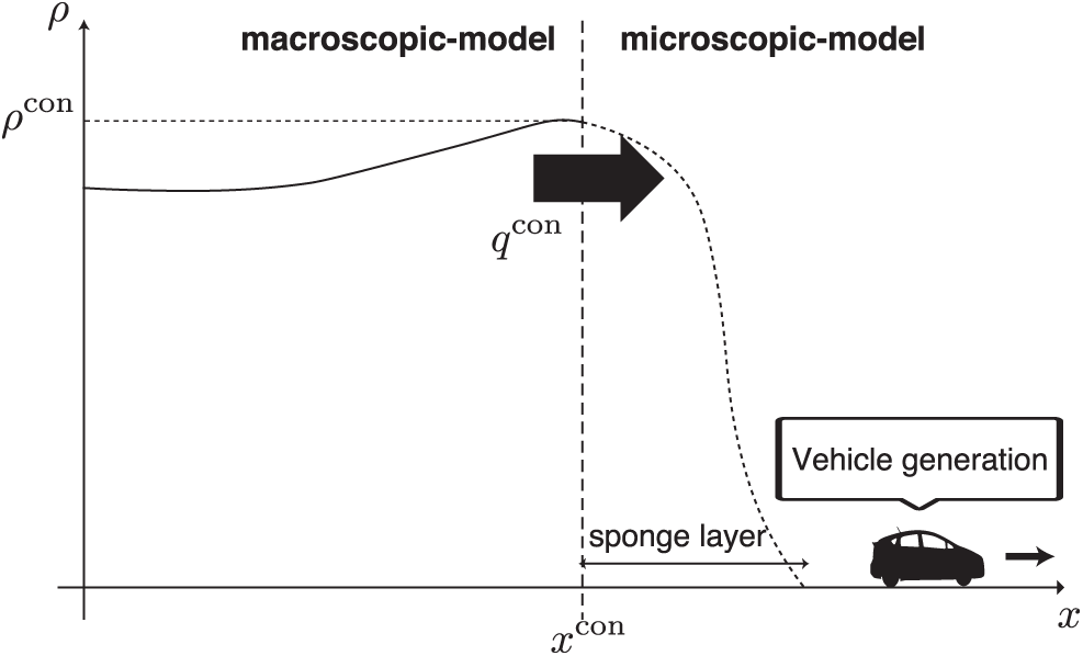
Figure 3: Connecting the Payne–Whitham model to the generalized force model

Next, consider the number of vehicles arising on the GFM side. For the GFM, we use a smaller timestep than for the PW model; denoting the ratio of timesteps by M, we have (Δ{t})NE = M(Δ{t})AG, where (Δ{t})NE and (Δ{t})AG are respectively the timesteps used for the PW model and for the GFM.

For the PW model, we denote by Ctotali the total accumulated number of vehicles that flow out before or on the nth timestep.

Ctotaln=∑i=1nCi (27)

For an arbitrary time t, the total accumulated number of outflow vehicles C(t) may be defined by piecewise linear interpolation among the values of Ctotali (i = 1, 2, …) for the appropriate timestep.

C(t)=Ctotaln+(Ctotaln+1−Ctotaln)(n+1)Δt−tΔt(nΔt≤t≤(n+1)Δt) (28)

As the PW model proceeds from step n to step n + 1, the GFM computation is performed M times; we refer to the mth of these computations as step n+mM (m = 1, 2, …, M). We denote by Dn+mM the number of vehicles generated within the GFM on step n+mM (m = 1, 2, …, M); this quantity may be computed as follows:

Dn+mM=⌊C(tn+mM)−Dtotaln+mM⌋Dtotaln+mM=∑i=1n−1∑j=1MDi+jM+∑j=1m−1Dn+jMtn+mM=(n+mMΔt) (29)

6  Numerical Experiments

6.1 Model Parameter Settings

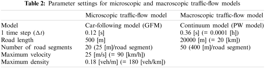
In this study, we use the parameter settings listed in Tab. 2 and conduct multiscale simulations of length 36000 s (10 h). Each simulation proceeds as follows. First, for each timestep in the macroscopic model, we write the time, velocity, density, and number of outflowing vehicles to an output file. On each of the fine-grained timesteps of the microscopic model, this file is re-read and its content reflected within the microscopic model. At this point in the macroscopic model simulation, we construct a graphical data visualization in which density and velocity values are represented respectively by the height and color of graphical data points, as shown in Fig. 4; in this figure, the the direction of traffic flow is from left to right, and the region in which the density appears to drop off is the sponge layer. Colder and warmer colors respectively indicate slower and faster velocities. From this visualization, we see that both the density and velocity attain spatially uniform configurations for this traffic flow.

We also generate graphical visualizations to illustrate results of the microscopic model simulation; an example is shown in Fig. 5. Note that individual vehicles are resolved in this model visualization. As indicated in the figure, vehicles occupy a single lane and proceed from left to right. The correctly implemented GFM shows the behavior of a vehicle running at maximum speed without any interaction between the vehicles. This corresponds to a basic validation issue in traffic simulation development, and we have already validated it.

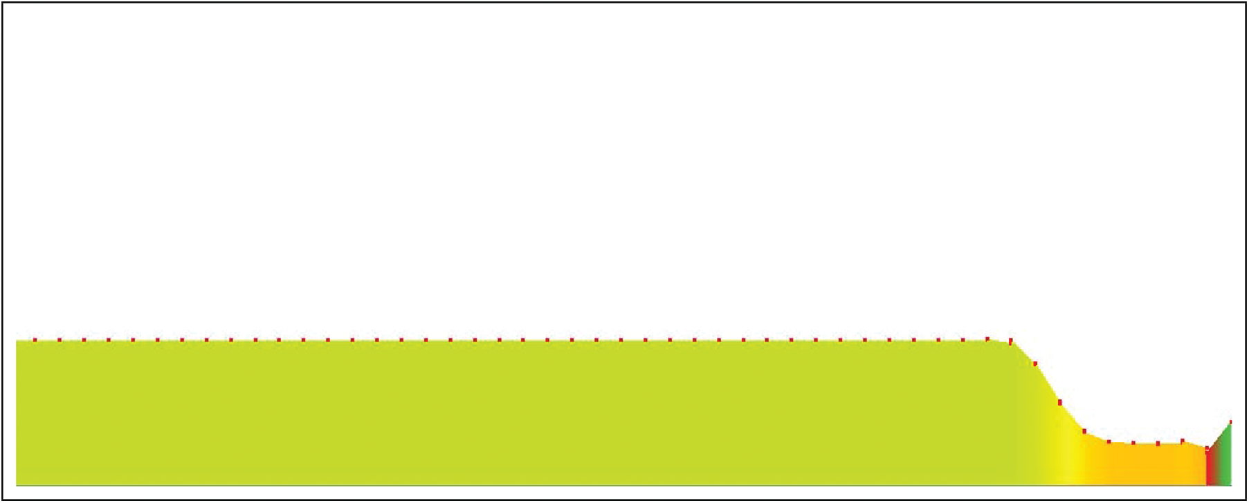
Figure 4: Graphical visualization of macroscopic traffic-flow model

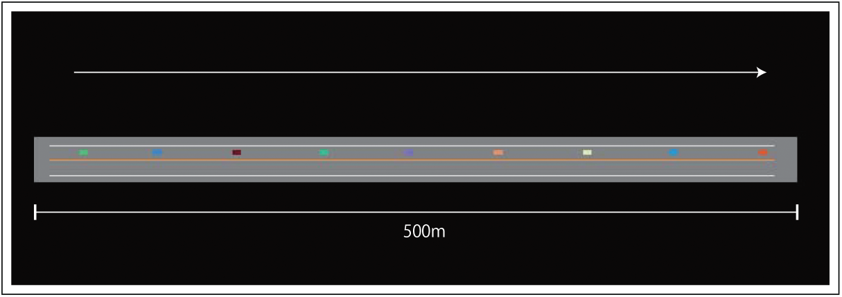
Figure 5: Graphical visualization of microscopic traffic-flow model

6.2 Conservation of Vehicles

Fig. 6 plots the number of vehicles flowing out from the macroscopic model and the number of vehicles flowing into the microscopic model. Evidently the outflow and inflow volumes are in agreement.

More precisely, whenever the number of outflowing vehicles—given by the product of the macroscopic-model traffic volume and the length of a single timestep—attains or exceeds an integer value, that number is input by the microscopic model as the number of inflow vehicles. Thus, the relationship between outflow and inflow counts may be stated more accurately in the form

=#{vehicles flowing into micromodel}+e, (30)

where 0 ≤ e ≤ 1, and this behavior is apparent upon more detailed scrutiny of the curves of Fig. 6, of which an enlarged portion is shown in Fig. 7.

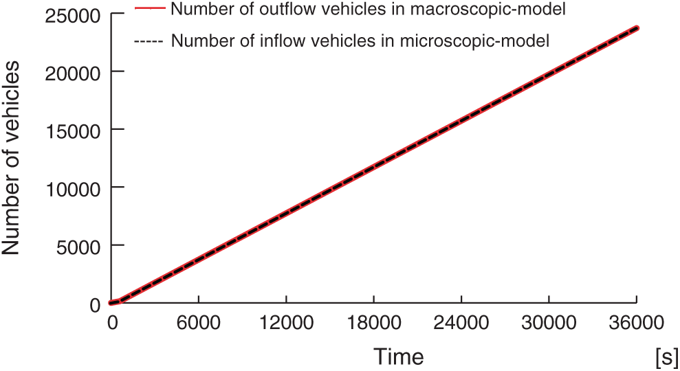
Figure 6: Numbers of vehicles flowing out of macroscopic model and flowing into microscopic model

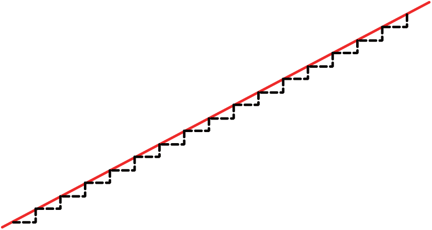
Figure 7: Enlarged view of the curves of the previous figure

We next compare the density distributions of the macroscopic and microscopic models. Fig. 8 plots the vehicle density for each discretization segment at simulation time t = 18000 s, the precise midpoint of the simulation.

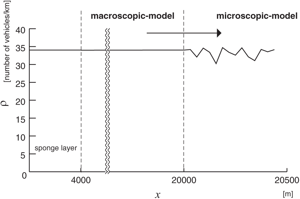
Figure 8: Density distribution of the multiscale traffic-flow model considered in this study

The section from 0 to 4 km is the sponge layer flowing into the macroscopic model, which in this case we have set to an inflow volume of 34 vehicles/km. On the other hand, the section from 16 to 20 km is the sponge layer for flowing out from the macroscopic model. To determine density values in the microscopic-model region, we obtain the positions of all vehicles on each segment, then evaluate a weighted average, with higher weights assigned to vehicles lying closer to segment centers, to obtain and plot quasi-density values for each segment.

6.3 Comparison of Computation Time

To compare computation times for various simulation models, we prepared three types of simulation and measured the computation time required to complete each: (a) our microscopic model alone, for which we prepared two timescales and conducted offline simulations; (b) the multiscale model proposed in this study, which combines a macroscopic and a microscopic model; and (c) a model consisting of a single simulation performed within our microscopic model. Results are tabulated in Tab. 3.

In this table, “Microscopic model (offline simulation)” refers to the total time required to complete two separate simulations of our microscopic model for roads of lengths 500 and 20000 m, whereas “Multiscale (micro + macro) model” refers to the time required to simulate the multiscale model proposed in this study, and “Microscopic model” refers to the computation time required to complete a single simulation of our microscopic model for a road of length 20500 m. For cases (a) and (c), when applying the microscopic model to wide target areas (specifically, the regions covered by the macroscopic model in case (b)), we chose parameter values in agreement with those used for the macroscopic model component of our multiscale simulations: a timestep of 0.36 s and a road of length 20000 m, discretized into 50 segments. For simulations in which the entire target region was analyzed via the microscopic model, we used a timestep of 0.12 s and a road length of 20500 m discretized into 75 segments.

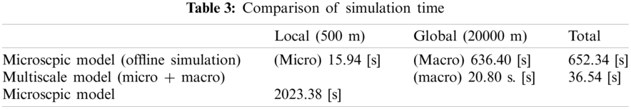
Tab. 4 lists the specifications of the workstation used for these calculations.

6.4 Discussion

We first analyze our simulation results to assess the extent to which the values of physical quantities are preserved by our methods for converting computational results between microscopic and macroscopic models. First considering vehicle counts from a microscopic point of view, Fig. 6 confirms that the number of vehicles flowing out of the macroscopic simulation agrees with the number of vehicles flowing into the microscopic simulation, validating the correctness of our conversion procedures. A second test is furnished by considering density values from a macroscopic point of view. From Fig. 8, identical density values were obtained in both the microscopic and macroscopic simulation regions, confirming that the density is continuous across the microscopic–macroscopic interface, although small fluctuations were observed in the figure, which were caused by discrete vehicle generation methods.

Possible explanations for the fluctuations on the microscopic side include (a) that the length of the discretization segments from which microscopic-model density values were computed was insufficiently long compared to the macroscopic model, and (b) the impact of the discreteness properties of the multiagent model. Nonetheless, although we clearly achieve an approximate conservation of density values between the two models, the densities are not in exact agreement. A little thought as to the origin of this discrepancy suggests that the difficulty may be due to the fact that the volume–density relation is not identical in the microscopic and macroscopic models. In the macroscopic traffic-flow model, the equilibrium velocity is given by the equation of [27], and this is multiplied by the density to yield the traffic volume:

In contrast, in the microscopic model, the number of vehicles is obtained by multiplying the traffic volume by the timestamp Δt to yield qΔt=vmρ(1−ρρm)Δt, from which the density may be reconstructed. Thus, the use of non-identical volume–density relations for the macroscopic and microscopic models may result in density discrepancies between the two models. In this study, we adjusted the macroscopic model to yield a volume–density relation close to that of the microscopic model; however, in future work, we hope to determine the volume–density relation in the macroscopic model from the basic diagrams of the microscopic model, thereby ensuring more accurate conservation of density.

Finally, with regard to computation times we note that replacing the microscopic model with the macroscopic model for simulating the greater part of the target area yields a computational cost reduction of 615.80 s—that is, nearly 10 min and 16 s—for a computation spanning 10 h of simulation time. That we failed to achieve even greater cost reduction in this case is probably due to the simplicity of our simulations, which involved only a single road and omitted complications such as traffic signals; we expect even larger computational savings for simulations of more realistic traffic-flow scenarios involving inter-vehicle interactions.

7  Conclusion

In this study, for the purpose of realizing high-precision traffic-flow simulations at low computational cost, we combined a microscopic traffic-flow model (the GFM, a car-following model) with a macroscopic traffic-flow model (the PW model, a continuous macroscopic model).

To discretize the PW model, we used a DGFEM, which not only offers robustness in the presence of discontinuities but also boasts outstanding stability properties. We also used a sponge layer to enhance stability in outflow/inflow regions. Then, we used our new model to simulate vehicle outflow from the macroscopic to the microscopic model and validated the accuracy of the results in two separate ways. First, measurements of the number of vehicles flowing out of the macroscopic model and flowing into the microscopic model confirmed that these quantities were in agreement at each timestep. Next, a comparison of density values obtained in the macroscopic model to post-conversion density values for the microscopic model confirmed that the requirement of density-value conservation was largely satisfied, indicating proper function of our multiscale model. Since there are countless combinations of DGFEM and multi-agent models, the proposed method may be applied to other combinations of macroscopic and microscopic models as well as the PW model and the GFM. The question of why macroscopic and microscopic density values were not in perfect agreement is a topic for future work, in which we hope to improve our procedure by using identical volume–density relations for the macroscopic and microscopic models.

A comparison of computational times confirmed that, thanks to the high speed of computations using the macroscopic model, our multiscale traffic-flow model yields high-quality results from simulations that complete in relatively little time.

In future work, we hope to study a reversed version of the multiscale model presented in this paper, in which quantities from a microscopic model are converted to a macroscopic model. To ensure vehicle outflow from a microscopic to a macroscopic traffic-flow model, we are considering methods for computing the mean velocity of vehicles arriving at the endpoints on each timestep, as well as techniques for converting vehicle counts to vehicle densities. In the macroscopic traffic-flow model considered here, one would like to use a sponge layer to yield fixed values for inflow and outflow, but this gives rise to fluctuations in values that had been held fixed. Thorough comparisons of the accuracy and applicability of advanced macroscopic models such as the Aw-Rascle-Zhang model [21,22] and higher-order methods of time integration such as strong stability-preserving Runge–Kutta method [30] will be important for future simulations of large-scale road networks.

We expect that successfully attaining these milestones would pave the way towards traffic-flow simulations that focus on subregions of wide-area systems.

Funding Statement: This work was supported in part by The Japan Society for the Promotion of Science (JSPS) KAKENHI Grant Nos. JP15H01785 and JP19H02377.

Conflicts of Interest: The authors declare that they have no conflicts of interest to report regarding the present study.

This work is licensed under a Creative Commons Attribution 4.0 International License, which permits unrestricted use, distribution, and reproduction in any medium, provided the original work is properly cited.