Computer Modeling in Engineering & Sciences

DOI: 10.32604/cmes.2021.014522

ARTICLE

Global and Graph Encoded Local Discriminative Region Representation for Scene Recognition

Chaowei Lin1,#, Feifei Lee1,#,*, Jiawei Cai1, Hanqing Chen1 and Qiu Chen2,*

1School of Medical Instrument and Food Engineering, University of Shanghai for Science and Technology, Shanghai, 200093, China
2Major of Electrical Engineering and Electronics, Graduate School of Engineering, Kogakuin University, Tokyo, 163-8677, Japan
*Corresponding Authors: Feifei Lee. Email: feifeilee@ieee.org; Qiu Chen. Email: q.chen@ieee.org
#Both authors contributed equally to this work
Received: 05 October 2020; Accepted: 19 May 2021

1  Introduction

Scene recognition is a basic computer vision task. Given a scene image, the computer can predict semantic labels according to its content. Compared with other classification tasks, such as object recognition, scene recognition is more challenging. In order to recognize a scene image, we not only need to care about its global layout but also the local scene features, which means specific objects appearing in the scene, i.e., detailed information. Moreover, another difficulty is that scene recognition suffers a huge semantic gap between the image content and labels, and recognition algorithms should learn to transfer local semantic clues to semantic labels. The translation is uncertain and hard to generalize, for example, “computer” can exist in “computer room” or “office”, and “table” can lead to predictions of “dining room” or “restaurant”. Scene recognition can provide prior knowledge for follow-up computer vision tasks such as object detection or event recognition.

In the past serval decades, scene recognition has drawn the attention of thousands of researchers and obtained numberless achievements. However, no matter how recognition methods change, they all depend on a fixed pattern, which Xie et al. [1] conclude as a general pipeline for image classification, also for scene recognition. Fig. 1 shows the general pipeline for scene classification.

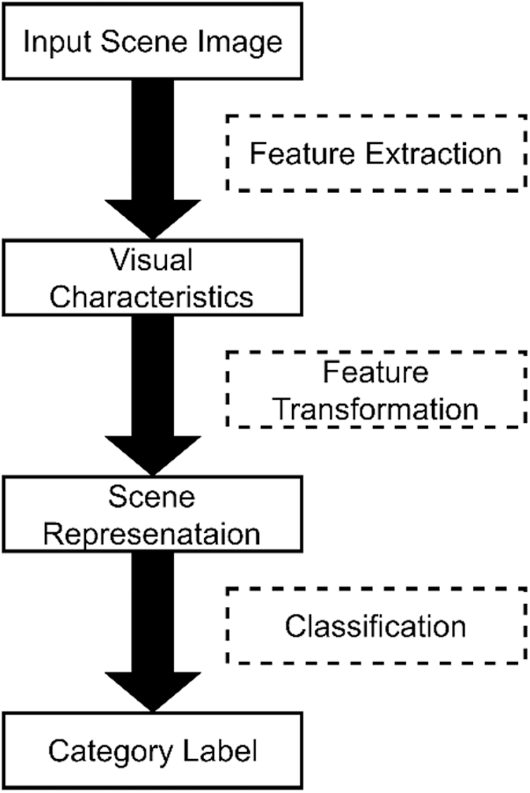
Figure 1: The general pipeline for scene classification

Scene recognition can also be divided into three steps, roughly but important. Given a scene image, the standard process is that we extract features firstly, then apply algorithms to transform the features into discriminative representations, and finally we train a classifier with the scene representation to predict scene labels. The evolution of scene recognition models mainly focuses on feature extraction and feature transformation.

In early stages, some hand-crafted features are constructed and used to extract low-level features. GIST [2], census transform histogram (CENTRIST) [3] and multi-channel CENTRIST [4] are global attribute descriptors carefully designed for scene recognition. For further improvement of scene recognition performance, some generic local visual descriptors including Scale Invariant Feature Transform (SIFT) [5], Histogram of Oriented Gradients (HOG) [6], Local Binary Patterns (LBP) [7] and Speeded Up Robust Features (SURF) [8] are utilized. These global or local descriptors can capture edge information, texture information, etc., which are low-level and unstable (susceptible to changes in illumination, scale or angle, etc.). Researchers have proposed some feature encoding methods to aggregate local descriptors into mid-level representation to solve this problem.

These methods can be classified as the second procedure in the general pipeline for scene recognition. Bag-of-Visual-Words (BoVW) [9] is proposed to calculate the distributions of local descriptors and form a global representation. Spatial Pyramid Matching (SPM) [10,11] is proposed to keep the spatial structure information of scene images by calculating the distribution of local descriptors falling into several pre-defined grids. Moreover, Locally Aggregated Descriptors (LAD) [12], Fisher Vector (FV) [13] are widely used. Even so, the mid-level scene representation generated after transformation is still inadequate for complex scene recognition, e.g., indoor scene categories, due to the limitation of discrimination of these local descriptors. Obviously, these feature transformation methods do not have the capability to fill up the huge semantic gap between hand-crafted descriptors and scene labels, and feature extraction methods are waiting for innovation.

As Deep Convolutional Neural Networks (DCNNs) [14] achieve a great success in ImageNet Large Scale Visual Recognition Challenge [15], convolutional features have replaced hand-crafted features in a variety of computer vision tasks, e.g., object classification [14], object detection [16], image retrieval [17], and of course scene recognition. Scene recognition benefits from discriminative, highly abstract and semantic convolutional features. Therefore, these conventional feature transformation methods [10–13] are combined with convolutional features, and a series of methods [18–21] are obtained, which are superior to hand-crafted methods. Multi-scale Orderless Pooling (MOP-CNN) [18] applies VLAD pooling of CNN activations extracted from multi-scale local image patches. Deep Spatial Pyramid (DSP) [19] constructs a deep spatial pyramid by partitioning on CNN feature maps in a way like SPM, then encodes each spatial region using FV with Gaussian kernel to form representation. In order to further reduce the semantic gap between scene representations and labels, semantic information is added to the feature transformation. Wang et al. [20] propose Vector of Semantically Aggregating Descriptor (VSAD) similar to FV and construct a semantic codebook to encode local image patches. Dixit et al. [21] propose semantic FV to encode pre-softmax CNN outputs which contains more semantic information than other previous layers. Different from the conventional feature transformation methods, Chen et al. [22] propose an advanced feature fusion algorithm using Multiple Convolutional Neural Network (MultiCNN) for scene recognition.

A scene image can be decomposed into three parts, i.e., global layout information, local scene or object information, and connections between them. Thus, MOP-CNN [18] performs dense sampling of scene images to ensure all discriminative local regions are included. Extracting features for dense sampling patches is obviously strenuous and redundant, and some works focus on locating or selecting discriminative patches among them [23–26].

In this work, we start from global attribute, and first construct a global representation using CNN activations. Then we focus on local discriminative regions and explore relation between with a graph model, a Graph Encoded Discriminative Region Representation (GEDRR) is introduced. In addition, we draw support of CNNs and employ convolutional activation as image features. According to LeCun et al. [27], we take consider of the dataset bias between object-centric datasets and scene-centric datasets. We propose a fusion method based on the multi-head attention [28] module, which can fuse CNN feature maps and object feature maps of the scene. All this above can be implemented in an end-to-end manner. In fact, we form a comprehensive representative for scene images, which is prevalent in current scene recognition models [18,20,25,27,29–31]. Vaswani et al. [29] propose representations with global features referring to the structure of the environment and local features capturing characteristics of common objects. Nascimento et al. [30] propose Fisher Convolution Vector to extract the local detailed information of convolutional features and directly involve fully-connect layer features to form the scene representation.

The main contributions of this paper are presented as follows:

1) We propose a scene recognition model called Global and Graph Encoded Local Discriminative Region Representation (G2ELDR2), which can produce a comprehensive representation for scene images. Our method not only introduces the global appearance representation, but also digs deeply into the local discriminative representation. In addition, the proposed model is end-to-end trainable.

2) We construct a Graph Encoded Discriminative Region Representation (GEDRR), which is supported by an online local discriminative region locator and a graph neural network. The local region locator is based on [25], but several changes have been made to fit our model. The significant and innovative changes make the local region locator an improved version of the original one. We also construct an undirected graph based on cosine similarity.

3) We propose a module using multi-head attention to fuse feature maps from two CNNs, which are pretrained on the object-centric dataset and the scene-centric dataset, respectively.

The rest of this paper is organized as follows. In Section 2, we take a brief review of related works. In Section 3, the details of proposed model are described. Section 4 describes the experimental set up and results, and evaluation experiments are also carried out in this section. Finally, we summarize our work in Section 5.

2  Related Works

In this section, we will briefly review works related to our method in several aspects.

2.1 CNNs and Scene Representation

Zhou et al. [26] propose LeNet-5 for handwritten digit recognition and the general structure of CNNs is designed. Due to the limitation of computing resources and massive training data, until 2012, AlexNet [14] with large-scale dataset ImageNet [15] has shown the great power of CNNs. CNNs begin prevalent in multiple computer vison tasks. The variants of CNNs including AlexNet [14], GoogLeNet [32], VGGNet [33], ResNet [34], etc.

CNNs can capture high-level, abstract and semantic information of images, so discriminative convolutional features replace the low-level hand-crafted features in scene image representation. [18,23,35–37] use ImageNet pretrained CNNs extract feature and gain good effect in scene recognition. However, ImageNet pretrained CNNs (object-CNNs) only respond to object cues of the input image. Because object cues are part of scene content, object-CNNs cannot comprehensively represent scene images. Also, LeCun et al. [27] point out that object-CNNs may ignore small-scale object of scene images. As the appearance of the large-scale scene dataset Places [38,39], the Places pretrained CNNs (scene-CNNs) is able to extract native scene-centric convolutional features. Places pretrained CNNs are a great promoting for development of scene recognition. These works [19,30,40] use scene-CNNs to extract features as scene representation, [20,21,25] take advantages of both (object-CNNs and places CNNs).

2.2 Attention Mechanism

Attention mechanism in artificial systems attempts to imitate human cognition. The power of human perception is that human beings can redistribute their attention to key parts of the information stream and focus on it. Attention mechanism is widely used in artificial intelligence tasks including natural language processing and computer vision. Herranz et al. [28] propose Transformer based on attention mechanisms for machine translation tasks. Tang et al. [41,42,43] proposed attention building blocks to provide support for modifying neural networks which is used in multiple computer vison tasks. The applications in subdivided fields of computer vison are listed as follows, image captioning [44], object detection [43,45], semantic segmentation [45,46], video classification [45].

Attention modules first reshape the input into independent units, then capture the long-range dependencies of them and obtain the global scale attribute coefficient for each unit. The coefficient is used to calibrate the value of each unit make some unit suppress others specifically, i.e., giving a large coefficient value to salient units. According to attention scope, the independent unit can be channel [41,42], spatial position in convolutional feature maps or both [43,44,46] (sequential [43,44], parallel [47]), word vector in natural language processing [41]. The ways of obtaining attention coefficients can be fully connected, matrix multiplication, and convolution. After these operations, softmax may be carried out to limit the range of coefficients into [0, 1]. [41,45,46] are matrix multiplication implemented attention, and we also adopt this form. In detail, we use the multi-head attention module in [41] and extend the self-attention to guided attention, which is used to fuse object-centric feature maps and scene-centric feature maps.

2.3 Discriminative Region Detection for Scene Recognition

Local discriminative regions are important cues for recognizing scene categories. The discriminative region may include objects, scene parts which are often occurrences in a scene. He et al. [35] propose to learn a part model from image patches by sparse dictionary learning and use the mid-level part model to build discriminative representation. In addition, Khan et al. [23] construct two sparse codebooks both in supervised and unsupervised manner from image patches, and use these two codebooks to encode image patches and then produce discriminative representation of a given scene image. In order to discovery discriminative region of a scene image, Lin et al. [24] introduce an improved spatial pooling method called Important Spatial Pooling Regions (ISPRs). ISPRs can learn discriminative part appearance containing useful visual cues to predict certain scene category. In the recent, Zhao et al. [25] propose Adaptive Discriminative Region Discovery (Adi-Red) to discover discriminative image regions with the help of Class Activation Mapping (CAM) [26], a class-specific image region locator. Adi-Red can capture classification clues related one specify scene category, and the detection is automatic and adaptive.

2.4 Class Activation Mapping

CAM proposed by Zhou et al. [26] shows its ability of localization. CAM can expose the implicit attention of CNNs on an image. It was designed to regularize training, but now it can be used in weakly-supervised object localization and visualizing CNNs. CAM can be applied to CNNs which perform classification task, use global average pooling after convolutional layers and have no fully connected layer expect the classification layer. CAM utilizes the knowledge from the classification layers to form a class activation map, which can highlight the active regions on the convolutional feature maps. In more detail, given a semantic label, CAM extracts related weights from the classification layer. Each position of the weight vector can be channel-wise corresponding to feature maps outputted by the last convolutional layers of CNNs (i.e., feature maps inputted into classification layer). Then CAM calculates the weighted average of the feature maps along the channel dimension. Each position of the generated class activation map can indicate the intensity of this location that is taken consider by the CNNs when CNNs are predicting a certain category. From above description, we also know that every category has their own class activation map, because different categories can activate different locations on feature maps. In addition, Grad-CAM [48] is proposed to obtain class activation map from any CNN-based models, the main idea is that Grad-CAM uses the gradients of any target category back forward from classification layer to the last convolutional layer as weights to produce the class activation map.

2.5 Graph Neural Networks

Graphs are a kind of non-Euclidean data structure which consist of nodes and edges. Graph Neural Networks (GNNs) are proposed to model this non-Euclidean structure and provide routines of message passing for each node based on deep learning. GNNs can model physics system, learn molecular fingerprints, predict protein interface, etc. [49], in the field of computer vision, GNNs can handle tasks including image classification [50], object detection [51], semantic segmentation [52]. In this work, we adopt Graph Convolutional Network (GCN) [53] to form node representation of local discriminative regions in scene images for scene recognition. Kipf et al. [53] introduce a simple and well-behaved layer-wise propagation rule for GCN. GCN is a variant of GNNs which uses convolutional aggregators to aggregate features from neighbor nodes in spectral domain. GCN can model the relationship of connected nodes via feature passing between one node and its 1st-oder neighborhood nodes. Zeng et al. [54] propose Semantic Regional Graph modeling framework which uses a semantic segmentation network to find semantic regions in scene images, then encodes the geometric information among semantic regions with GCN. In this work, we firstly construct a graph. In that graph, features extracted from discriminative regions are defined as nodes, the similarity among discriminative regions are defined as edges. After that, we perform GCN on the graph to explore the relationship among discriminative regions.

3  Proposed Method

In this section, we firstly present an overview of our proposed model and then give a detail description in the following subsections.

3.1 Overview

In this paper, we propose an end-to-end scene recognition framework G2ELDR2. We consider that global and local representations should be combined, because scene images contain global layouts and local scene features. The pipeline of G2ELDR2 is shown in Fig. 2. The purpose of our framework is to construct a comprehensive representation for scene images, which includes global object and scene attribute representation, and local discriminative region representation, i.e., GEDRR. The feature extraction relies on two pretrained CNNs. The rest of the framework focuses on feature transformation.

Feature maps from two pretrained CNNs are transformed to global representations by GAP. In addition, the two group of feature maps after flattening are sent to two multi-head attention modules and fused. The CAM generator takes scene-centric feature maps as input and produces center coordinates of discriminative regions which are used for cropping on fused feature maps. After cropping and GAP, the feature vectors are sent to GCN and GEDRR is formed. Finally, the comprehensive representation is sent to a fully connected classifier to predict scene categories. In the following subsections, we will give a detailed description of the G2ELDR2 framework.

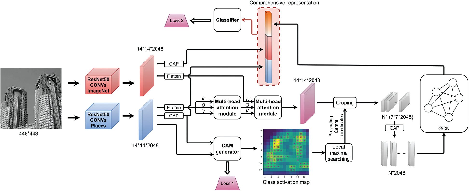
Figure 2: The pipeline of G2ELDR2. Two pretrained CNNs are used to produce scene-centric feature maps and object-centric feature maps. In the “comprehensive representation”, there are three vectors, two are global representations, and the last one is local representation which called GEDRR. In order to construct global representations, we simply perform Global Average Pooling (GAP) on the two feature maps and obtain two vectors, which represent global scene attributes and global object attributes, respectively. The formation of GEDRR is described as follows: first, feature maps from the two CNNs are flatten and sent to two multi-head attention modules for fusion, and the CAM generator gets scene-centric feature maps and generator center coordinates for cropping, then we crop on the fused feature maps and obtain the feature blocks which will be pooled using GAP and sent to GCN module, and finally we get GEDRR

3.2 Feature Extraction and Global Representations

We use two CNNs extract deep convolutional activations as initial features of scene images. The two CNNs are pretrained on Places [40] and ImageNet [15] respectively and so-called scene-CNN and object-CNN. We extract scene-centric features from scene-CNN as main representation to avoid dataset bias, we extract object-centric features as supplement to scene-centric features.

With the development of deep neural networks, CNNs become deeper and wider, and achieve better performance on many visual recognition tasks. In a series of variants of CNNs, we choose ResNet-50 [35] as the backbone of the CNN feature extractor. Compare with AlexNet, GoogLeNet, VGG, the architecture of ResNet-50 is deeper and has less parameters.

We remove the fully connected layer of CNNs, keep the convolutional layers. We take the entire image as input. We perform GAP on feature maps to obtain holistic and abstract global representations, i.e., scene-centric feature maps are transformed into global scene representation and object-centric feature maps are transformed into global object representation. However, due to the complexity and variants of scene images (especially indoor scene images), global representations are not discriminative enough. The recognition performance using only global features may not be good. The experimental results with only global features will be shown in Section 4. In order to improve the performance, we should combine global with local scale representations. We design discriminative and invariant GEDRR for local scales (The details of GEDRR will be descripted in Sections 3.3 and 3.4.).

3.3 Multi-Head Attention for Feature Fusion

To enhance the scene-centric features and fuse object-centric and scene-centric features, we adopt the attention function proposed by Vaswani et al. [29], the attention module is shown in Fig. 3.

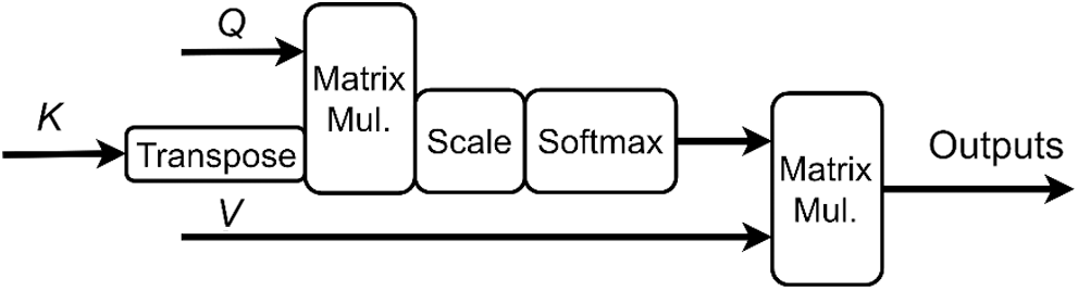
Figure 3: Scaled dot-product attention module (single head). The inputs of this module are a sequence of vectors, outputs are the same shape of the inputs. Q,K,Vare three copies of the inputs, called queries, keys, and values. Q and K go through a compatibility function, i.e., matrix multiplication, scale, softmax and produce weights which are used to compute the weighted sum of the values

As shown in Fig. 3, the inputs of attention module are Q,K,V corresponding to queries, keys, values, three copies of the inputs. K is firstly transposed and multiplied by Q. The process is a classic dot-product attention, to obtain the similarity values. Then the similarity values are turned into weights by softmax function. V is multiplied by the weights to calculate the outputs. Each vector of the outputs can be regarded as a weight sum of input vectors, the output vectors show the relationship between input vectors and global information of input vectors. The calculation process of the attention module can be concluded as follows:

Attention(Q,K,V)=softmax(QKTdK)V. (1)

In Eq. (1), dK is the dimension of K, 1/dK is scaling factor to prevent small gradients of softmax function because of large magnitude of the dot product results by vectors with large dK.

Based on the Scaled Dot-Product Attention module, we propose a method to apply self-attention module on scene-centric convolutional feature maps, so as to enhance the feature maps with spatial relationship and global information. The proposed method is shown in Fig. 4.

Actually, we use the multi-head attention module in [29] to obtain better recognition results, and Vaswani et al. [29] also suggest that it beneficial to project the Q,K,Vh times with different, learned linear projections and learn the rich, diverse attention patterns. In addition, the multi-head attention can search for different attention cues in the subspace. The multi-head attention module is shown in Fig. 5. Supposing that we have h heads, to get the input of each head, the original input vector is divided into h parts by h times linear mapping. Since there are three input vectors Q,K,V, 3h times linear mapping is required. After Scale Dot-Product Attention, h output vectors are concatenated to form a single vector, and then linear mapping is performed on it to form the final output of the multi-head attention module.

The procedure of Multi-head attention is as follows:

MultiHead(Q,K,V)=Concat(head1,…,headh)WO, (2)

headi=Attention(QiWiQ,KiWiK,ViWiv). (3)

where WiQ∈RdQ×dQi,WiK∈RdK×dKi,WiV∈RdV×dVi and WO∈RdQ=dK=di.

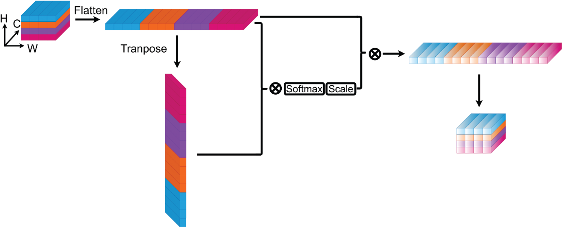
Figure 4: Scaled dot-product attention on feature maps (single head). We treat each position in H (Height) and W (Width) plane as input vector along C (Channel) axis. Then we flatten the spatial structure and get a vector sequence that can be handled by the attention module

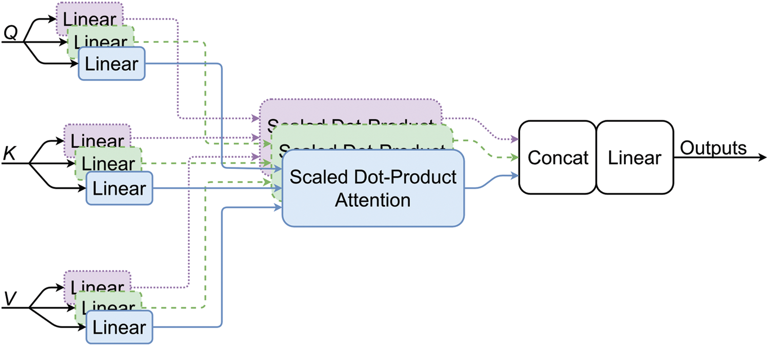
Figure 5: Multi-head attention with scale dot-product attention. Q,K,Vare linearly projected into Qi,Ki,Vi, suppose we have h heads, then dQ=h×dQi,dK=h×dKi,dV=h×dVi. Each head is sent to scaled dot-product attention module, after that we concatenate the results of multi-head and fuse by linear transformation

In this work, we introduce our double attention feature map fusion method. We adopt two multi-head attention modules (as shown in Fig. 2), the first one is self-attention, and the second is exogenous attention. The exogenous attention is to inject object information into scene feature maps. The former takes scene-centric feature maps as Q,K,V, while the latter takes object-centric feature maps as Q, enhanced scene-centric feature maps as K,V. The only difference between them lies that we change the queries Q from scene-centric feature maps to object-centric feature maps. Each position of the scene-centric and object-centric feature maps can be compared by the Scaled Dot-Product Attention. Thus, the difference and global attributes can be obtained and turned into weights to adjust the scene-centric feature maps. By the way, we perform a layer norm [55] on Q before inputting Q into the attention module.

3.4 Graph Encoded Discriminative Region Representation

Like Zhao et al. [25], our method finds the discriminative scene cues with the help of CAM [26]. We borrow the local maxima searching method from [25] and establish the first end-to-end discriminative region discovery module. Our proposed discriminative region detection module can generate class activation maps and find discriminative regions online with one forward propagation. Furthermore, we also make the feature extracting of discriminative regions online, i.e., we crop feature blocks directly on the feature maps by RoIAlign [56]. In addition, we construct an undirected graph, in which nodes are discriminative region features and edges are similarity between two regions. The undirected graph is sent to GCN to produce the GEDRR.

3.4.1 Class Activation Mapping

The class activation mapping utilizes the classification weights of single fully connected classification layers followed by convolutional layers. The way of generating class activation maps is the same of making predictions.

As shown in Fig. 6, we can see the only difference of class activation mapping and classifying is that whether perform GAP on the input feature maps. Thus, the result of class activation mapping can be turned to the predication result by GAP. Suppose we have feature maps fk(x,y),k∈[1,…,C] (x,y denote the position coordinate on the feature maps, k denotes channel number, suppose it has C channels), GAP can be concluded as follows:

gc=GAP(fk(x,y))=∑x,yfk(x,y), (4)

Let wkc denote classification weights for category c, to compute the prediction value Sc for category c, we have:

Sc=∑kwkcgc, (5)

Plugging Eq. (4) into (5), we have:

Sc=∑kwkc∑x,yfk(x,y)=∑x,y∑kwkcfk(x,y), (6)

In Fig. 6, we can see that there are two pathways for ① Feature maps transforming to ② Prediction value, i.e., ①-GAP-⨀⊕-② and ①-⨀⊕-GAP-②. So, noticing in Eq. (5), we change the position of GAP as the position changing of GAP in Fig. 6. Let Mc(x,y) denote the class activation map for category c, the calculation of Mc(x,y) can be given as:

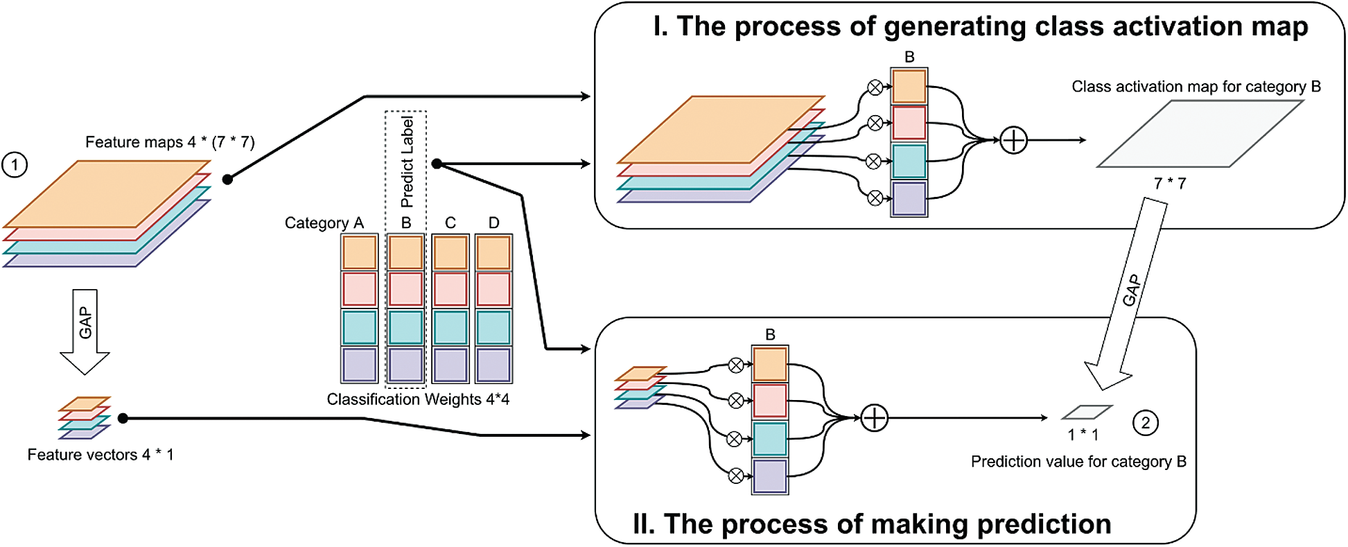
Figure 6: Comparing I. The process of generating class activation map and II. The process of making prediction. For simplify, we suppose that the size of the feature maps inputted into the classifier is 4×(7×7) and the size of the classification weights is 4×4. For a given category B, in I, each channel of the feature maps is multiplied by corresponding weight and then add the feature maps along channel axis; in II, feature vectors (GAP results of feature maps, each position corresponding to each channel) are multiplied by classification weights position-by-position and then sum

Mc(x,y)=∑kwkcfk(x,y). (7)

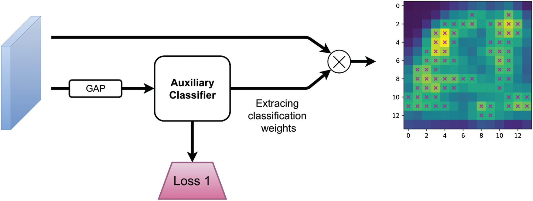
Figure 7: The online CAM generator. It includes a fully connected classifier and a multiplication operation. Inputs are scene-centric feature maps. After GAP, feature maps are sent into the classifier in where we extract the classification weights, then we multiply the feature maps by the classification weights as the operation in Fig. 6 I to get the class activation map

3.4.2 The Online CAM Generator

The CAM method proposed by Zhou et al. [26] has a limitation that CAM must apply on specific CNN architecture, i.e., convolutional layers-GAP-classifier. We cannot directly apply CAM on our model, because there are several transformations between the classifier and the last convolutional layers. In order to solve this problem, we introduce an auxiliary classifier that follows closely the last convolutional layers of scene-CNN as shown in Figs. 2 and 7, so that we can use the CAM module. The training signals given to the auxiliary classifier are the same with that given to the main classifier. The losses of the two classifiers are minimized together. For searching local maxima on the class activation maps, we normalize the values of class activation maps into [0,255].

3.4.3 Searches for Local Maxima on the Class Activation Map

On the class activation map, locations with high values means that these locations are discriminative. However, large quantities of redundant locations will be detected with above measurement. We should merge neigbhoring discriminative locations using a clustering algorithm or filter the discriminative locations like Zhao et al. [25], we choose the latter because of its simpleness and high efficiency.

The searching for local maxima is based on sliding window operation. As shown in Fig. 8, first we perform 0 padding on four sides of the class activation map, then we create a 3×3 sliding window with stride 1 and slide on each position of the class activation map. For each position on the class activation map, if its value is equal or greater than its 8 surroundings’ in the sliding window, it will be a local maximum. We get many local maxima after step I, but we need to filter the local maxima, because a part of them is redundant and another part of them have small values, i.e., less discriminative.

The filtering process is shown in Steps II, III in Fig. 8. The redundancy is defined as that maxima with the same value from overlapped windows. To reduce the redundancy, we keep one local maxima of the redundant maxima. Then, a threshold filtering is performed in Step III, experiments in Section 4 show how the threshold T affect the performance of our model.

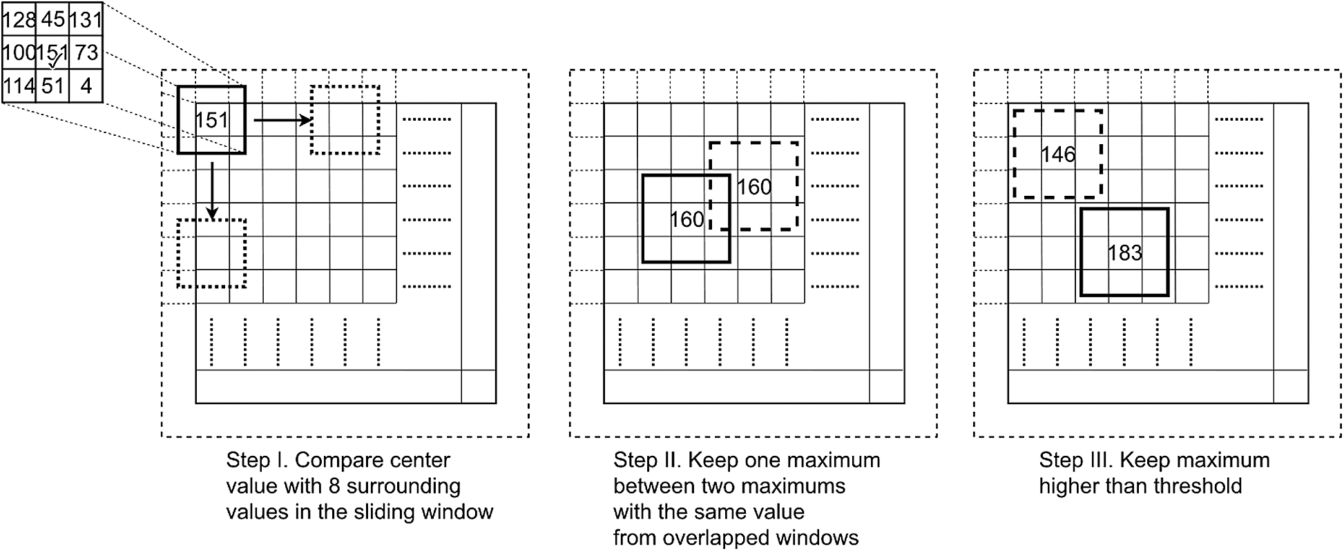
Figure 8: Main steps of searching local maxima. Before searching, we pad the class activation map with 0 on each side. There are three main steps: I. Find the maxima using a 3×3 sliding window, II. Delete the redundant maxima, III. Filter the maxima with a threshold

3.4.4 Extracting Features from Local Discriminative Region

The location of local maxima on the class activation map can be regarded as the center coordinate of the discriminative regions. Zhao et al. [25] extract local region features as follows. The image patches are cropped around the discriminative regions on the input image, and a three-scale image pyramid is constructed. Then, three pretrained CNNs are used and a quite a few times of forward propagations are performed to obtain convolution features, which is time consuming and computing intensive. According to the method proposed by Zhao et al. [25], a large disk space is also needed to save image patches and middle features. But in our proposed model, the feature extracting method is improved in time and space. We extract CNN features from all discriminative regions with one forward propagation, that is quite efficient and time saving. We also make the feature extracting end-to-end, so that the middle features do not need to be kept on the hard drive or other storage devices.

Once we get the discriminative regions, we directly crop on the feature maps using RoIAlign. We generate bounding boxes, which are centered on the coordinates of the local maxima. The size of bounding boxes is set to 7×7 and the output size of the RoIAlign is also 7×7, i.e., we crop 7×7 feature blocks from 14×14 feature maps. This operation is shown in Fig. 2 as “Cropping” module. The number of cropped feature blocks N is a hyperparameter that we search for it in Section 4.

3.4.5 Constructing Graph and Encoding with GCN

We get N discriminative regions per scene image from the class activation map. To capture the similarity between discriminative regions, we construct an undirected similarity graph G containing N nodes and N×(N−1)/2 edges. Node features are features from discriminative regions and edge features are the similarity between two nodes.

Node representations X and the adjacency matrix A is obtained to build the similarity graph G=(X,A). The process is as follows. Firstly, we perform GAP on N feature blocks and then get N feature vectors, which are regarded as node representations X so that X={X1,…,XN}. Then we calculate the similarity as adjacency matrix A∈RN×N using cosine similarity. We perform linear transformation and l2 normalization on the node representations to obtain the similarity:

Y=norm(XW), (8)

where W∈RdX×dX. For each element ai,j in A, we have:

ai,j=exp⁡(si,j)∑j∈{1,…,N}j≠iexp⁡(si,j), (9)

We perform GCN [53] on the similarity graph G to model the similarity relation of discriminative regions. Let G=(X,A) denote the similarity graph, where X denotes the node features and A denotes the adjacency matrix, the forward propagation function f of GCN can be represented as:

f(X,A)=D~−12A~D~−12XW, (10)

where A~=A+In, In is the identity matrix, A~ means the adjacency matrix with self-connections, D~i,j=∑jA~i,j, W is a trainable weight matrix. Activation function is often followed by the graph convolution, but we do not use the activation function because we use one graph convolutional layer. We perform max pooling on the graph convolutional result to get the final representation that we called it GEDRR.

3.5 Object Function

From Fig. 2, it can be noticed that our model has two losses, one is from the main classifier, we called it main loss Lmain and the other one is from auxiliary classifier of the CAM generator, we called it auxiliary loss Laux. During training, we simply add the two losses together then send them to the optimizer. Both losses are softmax cross-entropy losses. The objective function of our model can be formed as follows:

Lmodel=Lmain+Laux. (11)

4  Experimental Results

In this section, we evaluate the performance of our proposed scene model and compare it with state-of-the-art methods. Then, we show how to select key parameters by carrying out parameter analysis experiments. In addition, evaluation experiment results will be given to show the necessity of each component of our model.

4.1 Datasets

Scene 15 [57] contains more than 4000 grayscale scene images and has 15 categories including both indoor and outdoor scene images. We randomly choose 100 images for training and the rest for test in each category and it is a standard separation in comparing works.

MIT indoor 67 [58] is a widely used dataset for scene recognition. It has 15620 color images of indoor scene which is divided into 67 categories, each category has at least 100 images. We follow the standard evaluation separation that 80 images are for training and 20 images for test of each category.

SUN 397 [59] is a large-scale dataset for scene recognition. It contains 130519 images distributed in 899 categories, includes both indoor and outdoor scene images. The standard evaluation separation uses 397 well-sampled categories, 50 images are for training and 50 images are for test of each category. Xiao et al. [59] separated SUN 397 into ten different partitions, each of the partition has 50 images for training and 50 images for test. We evaluate our method on all the partitions and give an average result.

4.2 Implementation Details

Our model performs transformations on CNN features, we adopt two pretrained CNNs as feature extractor. We choose classic ResNet-50 as the backbone of the model. Two CNNs have different pretrained datasets, one CNN called scene CNN is pretrained on ImageNet [15] and the other called object CNN is pretrained on Places [40]. We remove the classification layers of pretrained CNNs while retaining the convolutional layers.

Before training our model, the auxiliary classifier in the CAM generator needs to be pretrained. We stack the auxiliary classifier on scene CNN, freeze the weights of convolutional layers and train the auxiliary classifier on the datasets. During training, the input images are resized into 256×256 and cropped 224×224 randomly and then randomly flipped in horizon for data augmentation. For Scene 15 and MIT indoor 67, the batch size is 32 and the number of epochs is 40. The learning rate is 0.01 and decayed every 10 epochs. For SUN 397, we train 60 epochs with batch size 50 and learning rate 0.01, also the learning rate decays every 15 epochs. During testing, the input images are resized into 224×224, we treat the test results as a baseline which shows the performance of single plain CNN.

The hyperparameters are listed in the follow. The shape of CNN features is 14×14×2048. The shape of class activation maps is 14×14. In the multi-head attention module, the number of heads h=32, dQ=dK=dV=2048, in each head, dQi=dKi=dVi=64. In local maxima searching, the threshold T=150, the number of feature blocks N=5. In GCN module, the number of the output channels of graph convolution is 2048.

During training of our model, the input images are resized into 480×480, randomly cropped 448×448 and then randomly flipped in horizon for data augmentation. For MIT indoor 67 and Scene 15, the batch size is set to 32, the epoch is 100. For SUN 397, the batch size is also set to 32 and the epoch is set to 45. We freeze the weights of object CNN so that the learning rate of object CNN is set to 0. The initial learning rate of our model except scene CNN and object CNN is set to 0.01, the initial learning rate of scene CNN is set to 0.0001 for prevent the learned weights of scene CNN from being undermined by large loss at the beginning of training. The learning rate decay is manually, on Scene 15, decaying at epoch 37, 53, 94, on MIT indoor 67, decaying at epoch 46, 56, 90, on SUN397, decaying at epoch 31, 41. During test, we perform 5-crop testing in [14], we report the average result of last 5 epochs. For SUN397 dataset, we report the average test result of ten partitions.

4.3 Results and Comparison with State-of-the-Art Methods

We evaluate our model on three scene datasets, Scene 15, MIT indoor 67 and SUN 397 to see the performance of the comprehensive representation for scene images. In addition, we make comparison with the state-of-the-art approaches to demonstrate the effectiveness of our model by using the accuracy on three datasets as the metric. As a model performs CNN feature transformation, it will only be compared with previous methods that using CNN features.

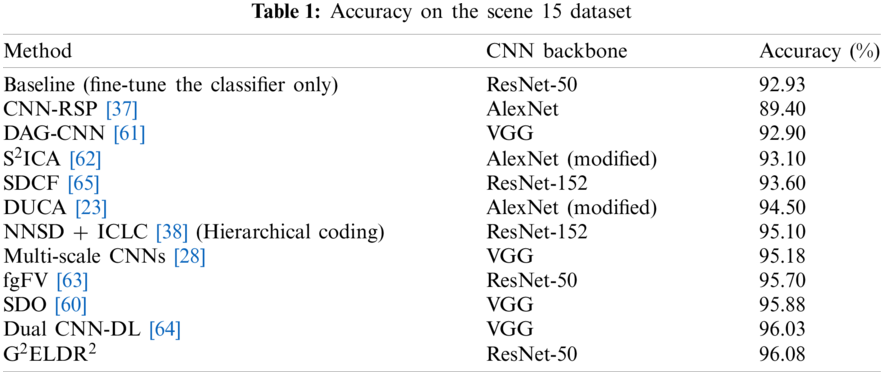
We report our comparison results on Scene 15 in Tab. 1. Our model achieves the state-of-the-art performance and outperforms recent scene recognition methods. By the way, an improvement of 3.15% is reported comparing with the plain CNN with one fully connected layer.

Among these approaches, Yang et al. [37] propose Randomized Spatial Pooling (RSP) to match the spatial layout information of scene images. Xie et al. [38] propose Non-Negative Sparse Decomposition (NNSD) to extract multi-scale features and Inter-class Linear Coding (ICLC) to learn discriminative features and ultimate representation for scene images. Cheng et al. [60] propose Semantic Descriptor with Objectness (SDO) that searching for representative and discriminative objects for each scene category and represent scene images with occurrence probabilities of objects. Yang et al. [61] propose Directed Acyclic Graph CNN (DAG-CNN) to capture multi-scale features by injecting the supervision signal into every convolutional layers. Hayat et al. [62] construct a novel Spatially Unstructured layer to modify CNNs for the reason of improving the robustness of CNNs against spatial layout deformations. Also, Hayat et al. [62] propose a pyramidal image representation to resist the scale variance of scene. Pan et al. [63] improve the traditional FV encoding method and propose the foreground FV (fgFV) method to separate foreground and background of scene and keep class-relevant foreground information. Liu et al. [64] also propose a dictionary learning method like that in [38], they propose the sparse dictionary learning layer and use it to replace the fully connected layers in CNNs.

The comparison results on MIT indoor 67 and SUN 397 are reported in Tab. 2. The results show that our model reaches the state-of-the-art performance in the two datasets. Comparing to the plain CNNs, our model exceeds about 3.16% and 2.55% on MIT indoor 67 and SUN 397, respectively. From Tab. 2, we also can find the importance of the feature transformation. For example, different transformation methods lead to a huge gap on experimental results based on VGG features. Zhao et al. [25] extract four-scale image patches and use four CNNs extract features, so their performance is slightly better than us on SUN397 dataset.

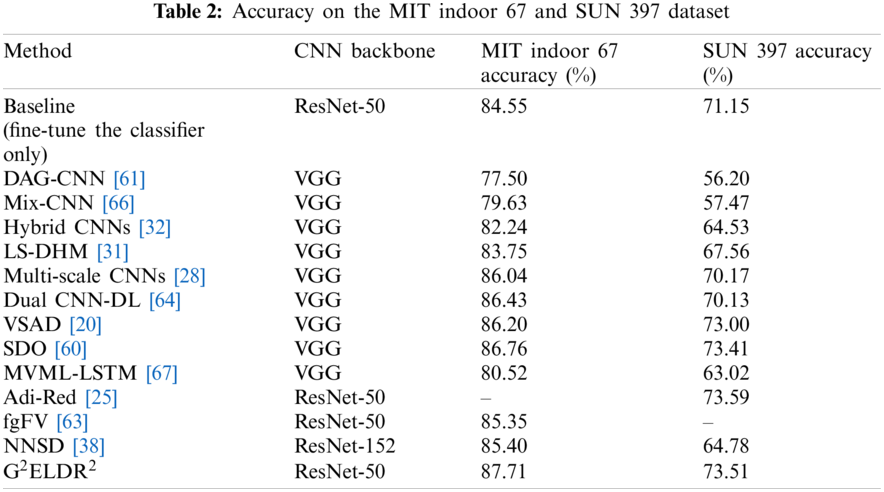
There are many different types of feature transformation methods in recent years. Xie et al. [32] transform two types of CNN features into hybrid representation, including FV encoded convolutional features, the part dictionary model encoded fully connected features and the fully connected features itself. Guo et al. [31] combine the fully connected features and FV encoded mid-level CNN features to represent scene images. Jiang et al. [66] propose a shared Locality-constrained Linear Coding method to encode different CNN features. Bai et al. [67] crop multi-view and multi-scale image patches and use Long Short-Term Memory Networks (LSTMs) to encode CNN features extracted from patches.

4.4 Hyperparameter Analysis Experiments

Two main hyperparameters in the GEDRR have a large influence on the model performance, i.e., the threshold T for local maxima filtering and the number of feature blocks N. We carry out experiments on MIT indoor 67 dataset to study how these hyperparameters affect the model performance. We choose 3 interval points of threshold T and block number N, i.e., T∈[100,125,150,175,200] and N∈[5,7,9], and combine these two groups of hyperparameters in pairs then train our model in the same way. The experiment results are shown in Fig. 9.

It can be seen from Fig. 9, the shape of the curves is almost inverted “V”, except N=9, which can be concluded that less representative regions are enrichment when T is small, discriminative regions may be discarded when T is large, the two situations may harm the model performance. When the threshold T>150, increasing the threshold T leads to a decrease in accuracy. Each level of the threshold has an appropriate set of the number of feature blocks N. Specifically, when T is small (T=125), it means that more discriminative regions may be kept. We use a large N (N=9), the performance may be good. In contrast, when T is large, a large N is not suitable for the model. That means, the selection of N depends on the selection of T, and a large N works only when the discriminative regions are sufficient. Combining the above description and experiments, we choose T=150 and N=5 and they work well.

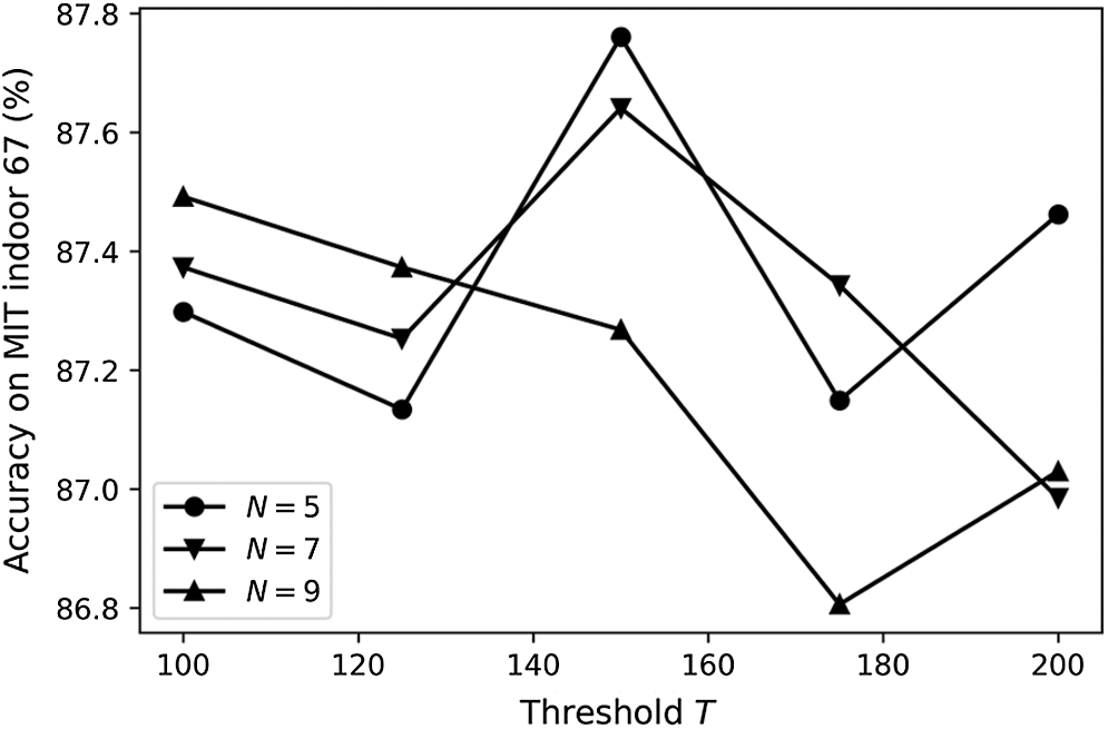
Figure 9: The test accuracy of proposed model on MIT indoor 67 dataset by different combination of two key hyperparameters, the threshold T and the number of feature blocks N

4.5 Ablation Study

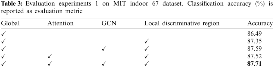
Our proposed model is a comprehensive system. From a macro perspective, we can divide our model into two parts, i.e., the global representation module and the GEDRR module. If we look into GEDRR module, it can be divided into two multi-head attention modules, that is, the Local Discriminative Region module and the GCN module. In order to prove the effect of each module in our model, we carry out a set of ablation experiments on MIT indoor 67 dataset.

We carry out 4 experiments in the first round. Experiment I: Remove the GEDRR module of the model. Experiment II: Remove two multi-attention modules and the GCN modules of the model. Experiment III: Remove the GCN modules of our model. Experiment IV: Remove two multi-attention modules of our model. Apart from above modifications, the experiment settings are the same as Section 4.2. The experimental results are shown in Tab. 3.

In order to prove the necessity of the two multi-head attention modules, we carry out 3 experiments in the second round. Experiment I: Global representation + local discriminative region representation + self-attention (the first attention module in Fig. 2). Experiment II: Global representation + local discriminative region representation + exogenous attention (the second attention module in Fig. 2). Experiment III: Global representation + local discriminative region representation + self-attention + exogenous attention. Except from above setting and N=9 in these experiments, the rest settings are the same as Section 4.2. The experimental results are shown in Tab. 4. We can see the necessity of both multi-head attention modules.

4.6 Discussions

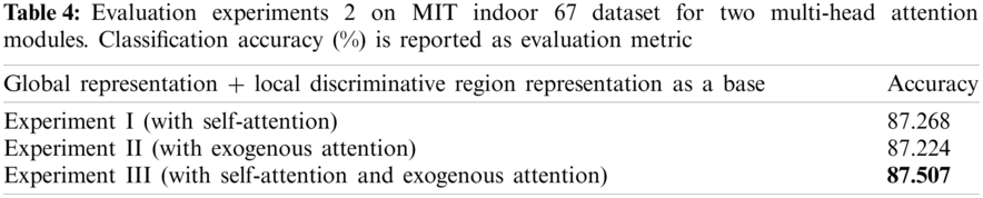
From Tabs. 1 and 2, we can conclude that our proposed framework achieves the state-of-the-art performance in scene recognition, and also proves that the necessity and feasibility of comprehensive representation. From Tabs. 3 and 4, we can see the contribution of each component of the framework. The great power of combining global layout representation and local detailed information shows that almost ∼0.9% improvement is achieved by comparing the model using only global representation with the model using both global and local representation. Optimal hyperparameters are found in Fig. 9. Despite the success of our framework, there is still a lot of room for improvement. For example, in the GEDRR module, future works can focus on improving the salient detection algorithm. A disadvantage in CAM-based salient detection is that the accuracy of the predict labels affects the accuracy of the salient detection, which will greatly affect the final recognition results. In addition, the multi-scale representation can be explored in future works because there are multi-scale patterns in a scene image, but we use only two scales. In short, the trend of scene recognition is comprehensive representation, which is effective and constant through the future development of scene recognition models.

5  Conclusions

In this paper, we propose a scene recognition framework called Global and Graph Encoded Local Discriminative Region Representation (G2ELDR2). The proposed model performs transformations on CNN features, uses the scene CNN and the object CNN to extract deep convolutional features, and then transforms these CNN features into a comprehensive representation in the global and local scale. The local representation is called Graph Encoded Local Discriminative Region Representation (GEDRR), which includes two multi-head attention modules, a local discriminative region extractor and a GCN module. Two attention modules are used to enhance scene information and fuse object information, and produce hybrid feature maps by them. The local discriminative region extractor is used to find the discriminative regions. The GCN module is used to model the sematic relationship between local discriminative regions. The experiments on three scene recognition datasets prove that our model can transform CNN features into a representative and discriminative representation for scene images, and our model have achieved the state-of-the-art performance.

Funding Statement: This research is partially supported by the Programme for Professor of Special Appointment (Eastern Scholar) at Shanghai Institutions of Higher Learning, and also partially supported by JSPS KAKENHI Grant No. 15K00159.

Conflicts of Interest: The authors declare that they have no known competing financial interests or personal relationships that could have appeared to influence the work reported in this paper.

This work is licensed under a Creative Commons Attribution 4.0 International License, which permits unrestricted use, distribution, and reproduction in any medium, provided the original work is properly cited.