Computer Modeling in Engineering & Sciences

DOI: 10.32604/cmes.2021.017211

ARTICLE

Multi-Material Topology Optimization of Structures Using an Ordered Ersatz Material Model

Baoshou Liu1,2, Xiaolei Yan1, Yangfan Li3, Shiwei Zhou4 and Xiaodong Huang3,*

1Fujian Key Laboratory of Automotive Electronics and Electric Drive, Fujian University of Technology, Fuzhou, 350118, China
2Key Laboratory of Advanced Technology for Vehicle Body Design & Manufacture, Hunan University, Changsha, 410082, China
3Faculty of Science, Engineering and Technology, Swinburne University of Technology, Melbourne, VIC 3122, Australia
4Centre for Innovative Structures and Materials, School of Engineering, RMIT University, Melbourne, VIC 3001, Australia
*Corresponding Author: Xiaodong Huang. Email: xhuang@swin.edu.au
Received: 22 April 2021; Accepted: 27 May 2021

1  Introduction

Topology optimization aims at finding optimal material distribution within the prescribed design domain and achieving the best performance of the structure. Since the seminar paper of Bendsøe et al. [1] in 1988, several topology optimization methods have been developed, including the homogenization method [2,3], the solid isotropic material with penalization (SIMP) method [4,5], the level-set method (LSM) [6–8], the bi-directional evolutionary structural optimization (BESO) [9–12]. With the recent development of additive manufacturing, multi-material structures can be comfortably fabricated and play an important role in practical engineering applications. The multi-material topology optimization has attracted increasing attention for designing lightweight structures.

Multi-material topology optimization traditionally seeks the best distributions of materials under multiple volume constraints so that the objective performance of the resulting multi-material structure is optimal. Sigmund et al. [13] and Bendsoe et al. [5] proposed a mixture rule of the multi-material model to characterize the distributions of materials in the SIMP framework. For instance, the three-material model containing two solid and one void materials can be described as Ee(ρ1e,ρ2e)=ρ1eP[ρ2ePE1+(1−ρ2eP)E2] for element e, where E1 and E2 are Young's modulus of two solid materials and ρ1e and ρ2e are artificial densities of element e. P is the penalty exponent. Naturally, all M-phase materials can be identified by total (M − 1) design variables and each material is generally restricted by the corresponding volume constraint [14–17]. In the level-set method, Wang et al. [18] introduced a “color” level set approach for multi-material topology optimization under multiple volume constraints and the subdomain of the k-th material is characterized as χk(Φ(x))=∏i=1m⁡HiIik, where Φ(x)=[Φ1(x),…,Φi(x),…,Φm(x)] is the vector of level set functions and Hi is the Heaviside function related to Φi(x). Iik is used as an index (0 or 1) and Hi1=H(Φi), Hi0=1−H(Φi). It indicates that only m level set functions are used to represent total of 2m-phases by the “color” level set method [18,19]. Besides, Huang et al. [20] extended the BESO method for achieving an optimal solution of multi-material structures, and the proposed method is further applied to the topological design of multi-material microstructures under multiple volume constraints [21–25]. Zhang et al. [26] proposed the moving morphable component (MMC) method to solve the multi-material topology optimization problem under multiple volume constraints using much fewer design variables and degrees of freedom. Other approaches have also been developed to solve the multi-material topology optimization problem, such as the phase-field method [27], the alternating active-phase algorithm [28,29], the bi-level hierarchical optimization method [30], the piecewise constant level set method [31,32] and the multi-material level set (MMLS) topology description [33]. The above multi-material topology optimization methods considered multiple material volume constraints, commonly called resource constraints.

In practical engineering applications, the total weight of a structure may be more concerned. This is a lightweight design, where the total mass should be reasonably adopted as a constraint or objective function for a multi-material design. However, when a single mass function is implemented with multiple design variables, some meaningless combinations of multiple design variables may occur and further bring some numerical difficulties for multi-material topology optimization. Yin et al. [34] introduced the peak function with SIMP method for the multi-material design using a single variable, but the horizontal zero slope of the peak function model has potential difficulties in numerical calculations. Gao et al. [35,36] developed a uniform multiphase materials interpolation (UMMI) scheme using multiple design variables. For example, a three-material UMMI model containing two solid and one void materials can be described by Ee(ρ1e,ρ2e)=ρ1eP(1−ρ2eP)E1+ρ2eP(1−ρ1eP)E2. The meaningless combination of two variables, i.e., ρ1e=ρ2e=1, an be possibly avoided, supposed that the penalty exponent P is large enough. The work also demonstrated that the multi-material topology optimization under a mass constraint might have multiple solutions. Zuo et al. [37] proposed an ordered SIMP interpolation using a single variable for solving multi-material topology optimization problems subject to a mass constraint and an additional cost constraint. Yang et al. [38] developed a BESO algorithm to find the optimal distributions of multi-materials under the total mass constraint by solving a series of two-material sub-problems.

The multi-material topology optimization using a single variable has an obvious advantage in saving computational cost [37]. However, the nonlinearity of the ordered-SIMP model could result in a local optimum as demonstrated in our late examples. Using the linear ordered-ersatz material model, this paper will develop a new multi-material topology optimization algorithm using a single variable based on the floating projection topology optimization (FPTO) method [39,40]. The FPTO method belongs to the element-based approach, but the structural topology is formed by the floating projection constraint, which simulates the 0/1 constraints of design variables. This provides the possibility for multi-material topology optimization using an ordered ersatz material model proposed in this paper. The remainder of this paper is organized as follows: Section 2 introduces the multi-material topology optimization problem and the ordered ersatz material model. In Section 3, the multi-material topology optimization algorithm is developed. Some 2D and 3D numerical examples are presented in Section 4 to verify the developed multi-material topology optimization algorithm, as well as its various applications. Finally, some conclusions are drawn in Section 5.

2  The Problem Statement and Material Model

2.1 Statement of the Topology Optimization Problem

Suppose that a multi-material structure is composed of M-phase materials within the design domain, where void is also as one material. Ei and ρi are Young's modulus and material density of the ith candidate material. Those candidate materials are sorted in the ascending order according to their normalized densities (ρN1<…<ρNi<…<ρNM) as

ρNi=ρi/ρmaxi=1,…,M(1)

where ρmax is the maximum density of all candidate materials, and the normalized Young's modulus of candidate materials is defined by ENi=Ei/EM. Topology optimization will build on finite element analysis with the fixed mesh and the design domain is discretized by a certain number of finite elements (e=1,…,NE) as shown in Fig. 1. Here, the normalized density xe is considered as a single variable of element e and will be relaxed to attain any value between xmin=10−6 and 1. xe=ρNi means element e is full of the ith material. Thus, the total mass of a multi-material structure, MT, can be expressed by

MT=∑e=1NE⁡(xeρmaxVe)(2)

where Ve denotes the total volume of element e. It can be seen that the elemental mass is linearly related to the single variable, xe, which overcomes the occurrence of meaningless design variables using multiple design variables.

Figure 1: Schematic illustration of the three-material design with the smooth boundary under the fixed-mesh finite element analysis

When the design domain is made up of multiple materials, as shown in Fig. 1. Ω=Ω1∪⁡Ω2∪Ω3 denotes the whole design domain in R2 or R3 and Ωi denotes the domain of material i. The topology optimization problem for minimizing the compliance of a multi-material structure can be stated by

{minx⁡C=FTus.b.K(x)u=FMT≤M¯T{xe=ρNiwhenxe∈Ωixe=ρNi−1whenxe∈Ωi−1ρNi−1<xe<ρNiwhenxe∈∂Ωi−1,ii=1,…,M(3)

where x={x1,…,xe,…,xNE} is the vector of design variables. K, u and F are the global stiffness matrix, nodal displacement vector and force vector, respectively. M¯Tis the constrained value of the total mass of the multi-material structure. To mathematically solve the above quasi-discrete topology optimization problem defined in Eq. (3), the elemental design variable, xe, is relaxed and assumed to attain any value between xmin and 1 and its material property is interpolated according to the following ordered ersatz material model.

2.2 Ordered Ersatz Material Model

For an element with the normalized density xe, it is necessary to define its material property, such as Young's modulus, for conducting the finite element analysis. In the traditional topology optimization method such as SIMP [14–17], the formation of structural topology traditionally originates from material penalization. Differently, the FPTO method [39,40] generates structural topology by employing the implicit floating projection constraint, which simulates the 0/1 constraints of design variables. Thus, the material interpolation can use the linear model, e.g., the ersatz material model. In the multi-material design, the ordered ersatz material model is proposed here. Considering that all candidate materials are well-ordered, i.e., EN1<…<ENi<…<ENM=1, the ordered ersatz material model is depicted as Fig. 2a. For an elemental design variable, ρNi−1≤xe≤ρNi, Young's modulus of element e can be linearly interpolated by

EeN(xe)=ENi−1+xe−ρNi−1ρNi−ρNi−1(ENi−ENi−1)(4)

where ENi and ENi−1 are the normalized Young's modulus of the candidate material i and i−1, respectively. Thus, the elemental stiffness matrix is expressed by

ke(xe)=EeN(xe)ke1(5)

where ke1 denotes the stiffness matrix of element e when fully filling with the heaviest material.

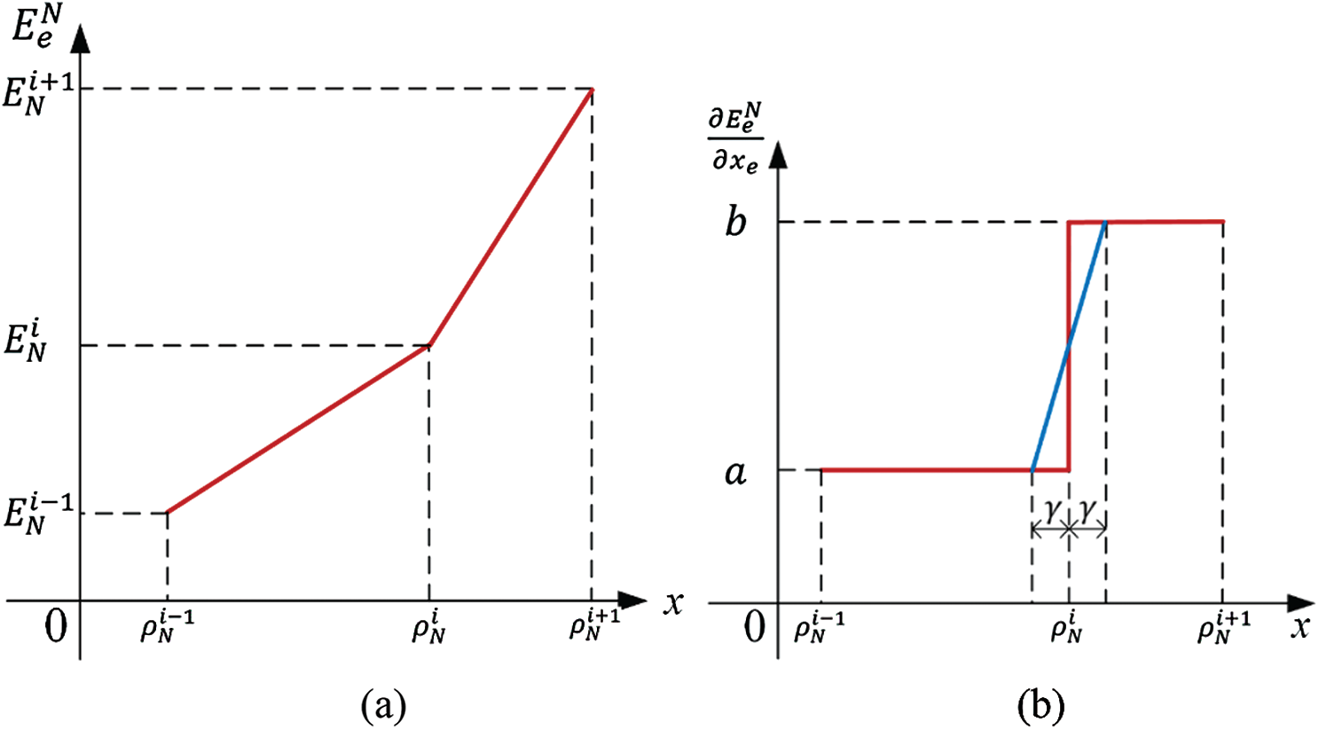
Figure 2: (a) Schematic diagram of the ordered ersatz material model containing three adjacent materials and (b) its linear transition scheme of the derivative near the point (ρNi,ENi) in Fig. 2a

However, such an ordered ersatz material model becomes non-differentiable at points, xe=ρNi as depicted by the red lines in Fig. 2b. To overcome this difficulty, a linear transition is assumed that the derivative continuously varies around those abrupt points as the blue line shown in Fig. 2b:

∂EeN∂xe={a=(ENi−ENi−1)ρNi−ρNi−1whenρNi−1≤xe≤(ρNi−γ)b=(ENi+1−ENi)ρNi+1−ρNiwhen(ρNi+γ)≤xe≤ρNi+1a+b−a2γ(xe−ρNi−1)when(ρNi+γ)≤xe≤(ρNi+γ)(6)

where γ=0.02 is used in this paper. Thus, the derivative, ∂EeN∂xe, becomes continuous over the whole range from xmin to 1.

3  Multi-Material Topology Optimization Algorithm

3.1 Update Scheme

To consider the mass constraint defined in Eq. (3), the objective function can be modified by introducing a Lagrange multiplier as

min:f=C+Λ(MT−M¯T)(7)

where Λ≥0. For the convenience of numerical implementation, the objective function can be further modified by

min:f=(1−λ)C+λ(MT−M¯T)(8)

where 0≤λ≤1 and therefore Eq. (8) is equivalent to Eq. (7) for the minimization operation. Thus, the optimality criterion of the problem can be expressed by

∂f∂xe=(1−λ)∂C∂xe+λ∂MT∂xe=0(9)

where the sensitivity of the compliance can be easily derived by using the adjoint method.

∂C∂xe=−uT∂K∂xeu=−ueT∂ke∂xeue=−∂EeN∂xeueTke1ue(10)

According to Eq. (2), the sensitivity of the total mass fraction is straightforward

∂MT∂xe=ρmaxVe(11)

Meanwhile, the sensitivity of the compliance is averaged with its value in the previous iteration to damp the update of the design variables

∂Cl∂xe=∂Cl∂xe+∂Cl−1∂xe2whenl>1(12)

where l is the current iteration number.

The optimality criterion in Eq. (9) can be further expressed by

Al≡(1−λ)∂Cl/∂xe∂MT/∂xe+λ=0(13)

Thus, the design variable of element e is updated by

x1,e=xel−1(1−Al)(14)

where the negative sign before Al denotes the search direction. It can be seen that x1,e=xel−1 when the optimality criterion is satisfied, i.e., Al=0. To overcome the checkerboard pattern and mesh-dependence problem [41], the heuristic density filter is employed, and the design variable is then modified by

x2,e=∑wje⁡x1,e∑wje(15)

where the wje is the linear weight factor as

wje={rmin−rjeifrje<rmin0ifrje≥rmin(16)

where the rje is the distance between the jth element and the eth element. rmin is the specified filter radius by the user.

In the traditional solid/void topology optimization, the implicit floating projection constraint simulates 0/1 constraints of design variables and further modifies the design variables after filtering. In the multi-material design, all design variables should be constrained to the discrete values, ρNi (i=1,2,⋯,M). Therefore, any design variables between ρNi and ρNi+1 are further modified by the following Heaviside function.

xel=ρNi+(ρNi+1−ρNi)tanh(β⋅(thi−ρNi))+tanh[β⋅(x2,e−thi)]tanh(β⋅(thi−ρNi))+tanh[β⋅((ρNi+1−thi)](17)

where β controls the steepness of the Heaviside function and thi is the ith threshold. Note that the projected design variable, xel is between ρNi and ρNi+1 but may be close to ρNi or ρNi+1 depending on the value of β. The threshold is determined by ensuring that the summation of x2,e between ρNi and ρNi+1 equals to the summation of xel between ρNi and ρNi+1. The projection function is applied to any two adjacent materials, and xel is therefore updated by M − 1 projection functions. Then, the move limit δ, the upper and lower bounds of the design variables are applied by xmin≤xel−1(1−δ)≤xel≤xel−1(1+δ)≤1. The Lagrange multiplier λ is determined by ensuring that the design variables, xl={x1l,⋯,xel,⋯,xNEl} satisfy the given mass constraint. This can be easily accomplished by using the bi-section method.

With the increase of β, the design variables are gradually pushed towards ρNi and a clear multi-material topology is created. For the robustness of the algorithm, β starts from a small positive value, e.g., 10−6, and increases with Δβ=1. For a given β, the solution converges when the variation of the objective function over the last 10 iterations is small enough, as defined by the following equation.

ϵ=∑k=1Q⁡|Cl−k+1−Cl−Q−k+1|∑k=1Q⁡Cl−k+1≤0.001(18)

where ϵ is the allowable convergence tolerance and Q is set as 5. Meanwhile, the β will stop increasing once the optimized result is close to a smooth design with a clear interface between two adjacent materials, which will be explained in the next section.

3.2 Representation of a Solution with Smooth Interfaces between Two Adjacent Materials

Once the algorithm is convergent for a given β, we should check if the desired solution is achieved. Similar to the FPTO method for a solid/void design [39,40], the resulting design variable x is linearly interpolated into the whole design domain, x(x,y). The M − 1 level-set functions are constructed for distinguishing the M-phase materials in the multi-material design. The ith level-set function is defined to identify the interface or boundary between the ith and i + 1th materials.

ϕi(x,y)=x(x,y)−lsiforρNi≤x(x,y)≤ρNi+1(19)

where lsi is the threshold, and the area or volume above and below the zero level-set can be assumed as the heavier and lighter materials, respectively.

{ϕi(x,y)>0formateriali+1ϕi(x,y)=0fortheinterfacebetweenmaterialsiandi+1ϕi(x,y)<0formateriali(20)

The threshold, lsi, is determined by ensuring that the total mass of materials\; i and i+1 identified by this level-set function is equal to the summation of the design variables between ρNi and ρNi+1. Finally, we identify all interfaces between any two adjacent materials and thus the whole design domain is divided into many regions representing the multiple materials, as depicted in Fig. 1.

Obviously, the above level-set functions are purely based on imaging processing and the resulting multi-material design may be far different from the element-based design expressed by the design variables, x. To check the difference between the multi-material design and the element-based design, we project the resulting multi-material design back to the fixed mesh and re-calculate the density of each element. If an element is fully occupied by material i, the density of the element is assigned with x¯e=ρNi. If an element is occupied by two adjacent materials, we calculate the volume fractions of each material inside the element and then x¯e is assigned with the homogenized density. According to the ordered ersatz material model, the compliance of the multi-material design, C¯, is calculated by one additional finite element analysis. The difference between the multi-material design and the element-based design can be measured by

τ=|C−C¯C|(21)

where C denotes the compliance of the element-based design. If τ is larger than 0.01 which means there is a large difference between the resulting multi-material design and the element-based design, and β increases with Δβ for further optimization as described in the last section. Otherwise, β keeps unchanged.

4  Results and Discussion

In this section, several 2D and 3D numerical examples are presented to demonstrate the effectiveness of the proposed multi-material topology optimization algorithm. It is assumed that Poisson's ratio of all candidate materials is v = 0.3.

4.1 Multi-Material Cantilever Beam

As shown in Fig. 3, a typical cantilever beam composes of two solid materials (m1, m2) and one void material. The design domain is discretized with 120 × 80 four-node plane-stress elements. A vertical concentrated force F=10 kN is applied at the middle of the right side of the beam and the left side is fully fixed. The material properties of the solid materials are E1=60GPa, ρ1=500kg/m3, E2=100GPa and ρ2=1000kg/m3. The constraint of the total mass is M¯T=6×103kg.

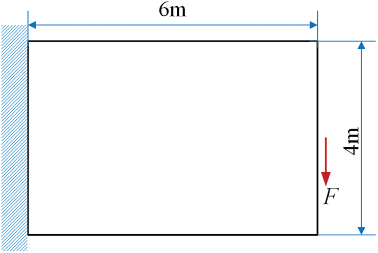
Figure 3: Design domain, dimensions and boundary condition of a cantilever

The optimized multi-material design is shown in Fig. 4a, whose compliance is 49.63 Nm, and the volume fractions of m1 and m2 are 42.2% and 3.9%, respectively. It can be seen that the stiff material (m2) appears around the concentrated load and the concerns of the fixed boundary to resist high stresses. The optimized design is mainly composed of material 1 (m1) since its stiffness-density ratio is higher than that of material 2. In order to verify the optimized multi-material design, the traditional solid-void designs using m1 or m2 only are shown in Figs. 4b and 4c. The compliances of those solid-void designs are 52.29 Nm and 59.41 Nm, respectively, while the total mass of those designs is still 6×103kg. It well indicates that the multi-material design is better than those of the traditional solid/void designs because the multiple materials expand the design space.

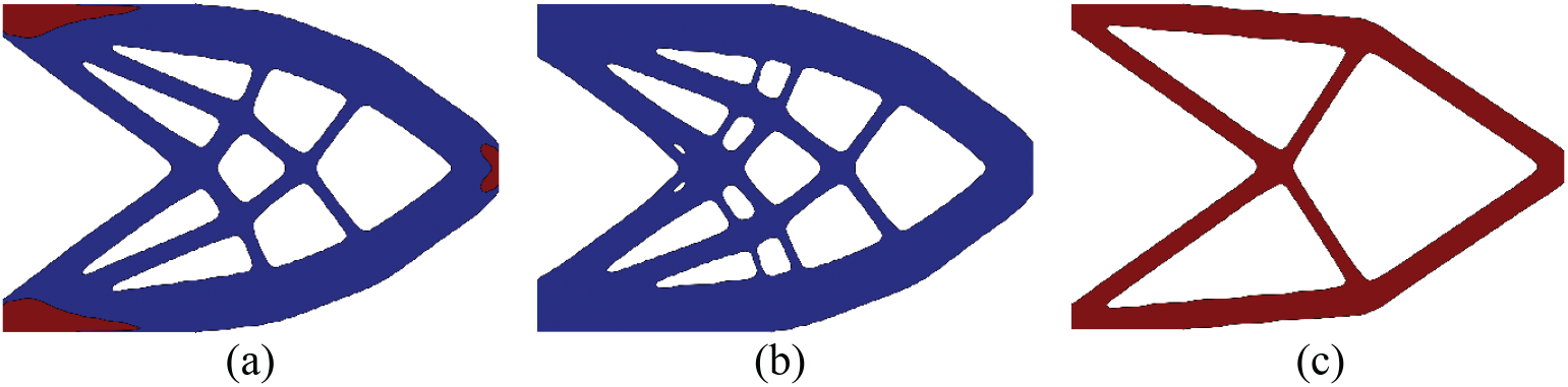
Figure 4: Comparison of the optimized designs where m1 and m2 are represented by blue and red colors, respectively. (a) the multi-material design and its compliance is 49.63 Nm; (b) the solid-void design using m1 and its compliance is 52.29 Nm; (c) the solid-void design using m2 and its compliance is 59.41 Nm

Fig. 5 shows the iteration histories of the compliance, topology and β for the multi-material design. Initially, the compliance stably decreases and achieves its minimum at iteration 66. However, the corresponding design contains a large volume of “grey” elements and the design variables are far away from discrete values, 0, 0.5, or 1, as required in the problem. Thereafter, β increases so that the corresponding floating projections simulate stricter discrete constraints of design variables. As a result, design variables gradually aggregate to the specified discrete values and the compliance increases due to such stricter constraints imposed to design variables. When β=7, a clear multi-material topology is formed. However, its compliance is still away from that of the representative design and therefore β further increases. When β=10, the compliance of the element-based design is close enough to that of the smooth design (τ=0.89%), and the whole optimization is thus stopped with 219 iterations. Fig. 5 also indicates that the formation of structural topology attributes to the increase of β, that is, the adoption of the floating projection constraint.

Figure 5: Iteration histories of the compliance, topology and β during the multi-material design with M¯T=6×103kg

4.2 Multi-Material Designs of a Simply Supported Beam

This example shows the multi-material design for a 2D beam as shown in Fig. 6 under the total mass constraint, M¯T=5.4×103kg. The design domain is discretized with total 120×60 four-node plane-stress elements. Three concentrated forces are applied at the 1/4, 1/2 and 3/4 of the bottom edge and F=10kN. The structure is assumed to be composed of three solid materials (m1, m2 and m3) and their material properties are listed in Tab. 1. In the final design, those three materials can be represented by blue, red and black colors, respectively.

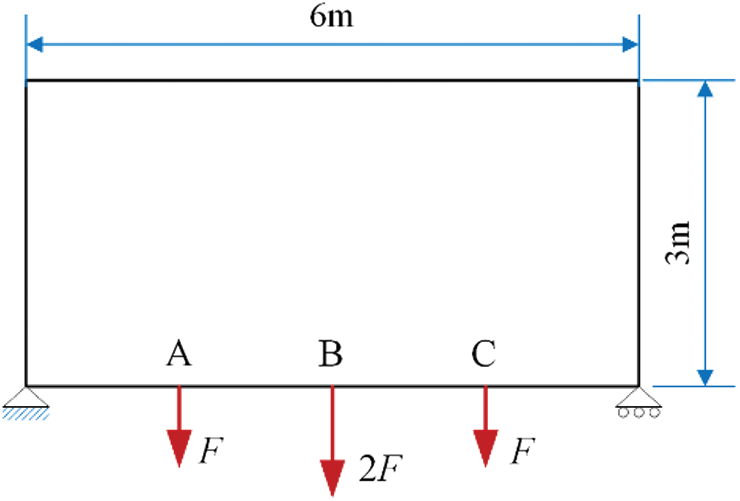
Figure 6: Design domain, dimensions and boundary condition of a simply supported beam

Under the given mass constraint, Fig. 7 shows the optimized results using the different combination of candidate materials: (a) void, m1, m2 and m3; (b) void, m2 and m3; (c) void, m1 and m3; (d) void, m1 and m2; (e) void and m1; (f) void and m2; (g) void and m3. In Fig. 7a, the compliance of the optimized design using all of the candidate materials is 193.32 Nm, which is the lowest one compared with other designs. The stiff material (m3) mainly distributes near the locations of concentrated forces and supports. The volume fraction of m1 is larger than that of m2 and m3 because its stiffness-density ratio is the highest. In these designs composed by two solid materials, as shown in Figs. 7b–7d, their corresponding compliances are 207.17 Nm, 195.49 Nm and 208.17 Nm, which are higher than that of the previous design. The compliances of the traditional solid/void designs shown in Figs. 7e–7g are 264.08 Nm, 221.63 Nm and 232.03 Nm, respectively. Therefore, the compliance of the multi-material design in Fig. 7a has the minimum compliance, which also indicates the advantage of optimally designing structures using multiple materials and the effectiveness of the proposed multi-material topology optimization algorithm.

Figure 7: Optimized designs under M¯T=5.4×103kg. (a) the multi-material design using m1, m2, and m3, and its compliance is 193.32 Nm; (b) the multi-material design using m2 and m3, and its compliance is 207.17 Nm; (c) the multi-material design using m1 and m2, and its compliance is 195.49 Nm; (d) the multi-material design using m1 and m2, and its compliance is 208.17 Nm; (e) the solid-void design using m1, and its compliance is 264.08 Nm; (f) the solid-void design using m2, and its compliance is 221.63 Nm; (g) the solid-void design using m3, and its compliance is 232.03 Nm

Different from the ordered SIMP method, the structural topology is formed by the floating projection constraint in the proposed multi-material topology optimization algorithm. For the comparison, the above example is re-calculated using 100 × 50 rectangular elements and F = 1, which are the same to that in the reference [37]. The properties of the candidate materials are listed in Tab. 2 and the constraint of the mass fraction (the ratio between the total mass and its possible maximum) is 0.4. Fig. 8a shows the optimized result by the proposed multi-material topology optimization algorithm and Fig. 8b is reproduced from the reference [37] by using the ordered SIMP model. The compliance of the current design, 194.4, is much lower than that using the ordered SIMP model, 217.2. It can be seen that the distributions and volumes of candidate materials are totally different. This example further demonstrates the effectiveness of the proposed algorithm, which could achieve a better solution compared with the existing order-SIMP method.

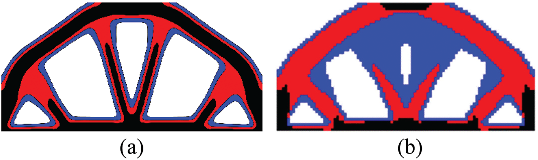
Figure 8: Optimized designs resulting from different material models: (a) the multi-material optimized design from the proposed algorithm using the order-ersatz material model, and its compliance is 194.4; (b) the optimized multi-material design using the ordered SIMP model in the reference [37], and its compliance is 217.2

4.3 Lightweight Designs of a Simply Supported Beam Subject to Displacement Constraints

In practice, it preferably achieves a lightweight structure under single or multiple displacement constraints. The proposed multi-material topology optimization, similar to the FPTO method [39], can be easily extended to solve such a problem, which can be mathematically stated as

{minx⁡MTs.b.K(x)u=Fuk≤uk∗k=1,…,Nc{xe=xiwhenxe∈Ωixe=xi−1whenxe∈Ωi−1xi−1<xe<xiwhenxe∈∂Ωi−1,ii=1,…,M(22)

where ukand uk∗ are the nodal displacement at point k and its corresponding upper constraint. Nc is the number of specified displacement constraints.

Taking the simply supported beam shown in Fig. 6 as an example, the vertical displacements at the point A, B and C are restricted as uA=uC≤4mm and uB≤5mm. Fig. 9 shows the optimized designs under the various combinations of the candidate materials listed in Tab. 1: (a) void, m1, m2 and m3; (b) void, m2 and m3; (c) void, m1 and m3; (d) void, m1 and m2; (e) void and m2; (f) void and m3. The final minimized mass of those optimized designs is also listed in Fig. 9, where the specified displacement constraints are strictly satisfied. The results show that the total mass from the optimized design in Fig. 9a has the least one compared with other optimized designs shown in Figs. 9b–9f. This result is reasonable because the optimized design in Fig. 9a allows using all candidate materials so that the design space is maximum compared with other cases. Comparably, the total mass of the traditional solid-void designs shown in Figs. 9e and 9f is larger than that of the multi-material designs, which demonstrates the advantage of designing structures using multiple materials. In all multi-material designs, the stiffest material is always allocated near the locations of the concentrated loads and supports to resist high stresses. The material with the highest stiffness-density ratio has the maximum volume fractions compared with that of other solid materials. In all cases, the FPTO method provides smooth interfaces between adjacent materials in the optimized designs.

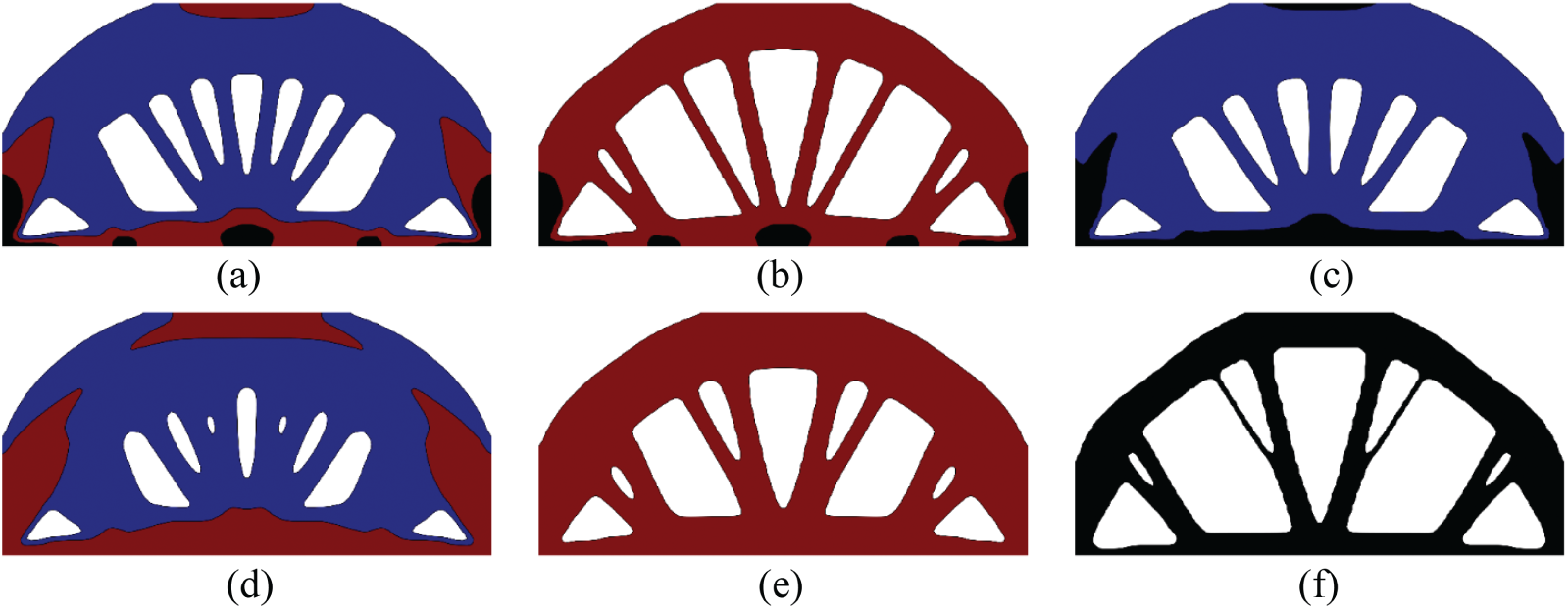
Figure 9: Optimized designs for minimizing the mass subject to three displacement constraints, uA=uC≤4 and uB≤5. (a) the multi-material design using void, m1, m2 and m3, and the final mass is 6.04×103kg; (b) the multi-material design using void, m2 and m3 and the final mass is 6.63×103kg; (c) the multi-material design using void, m1 and m3, and the final mass is 6.15×103kg; (d) the multi-material design with void, m1 and m2, and the final mass is 7.12×103kg; (e) the solid-void design using void and m2, and the final mass is 7.77×103kg; (f) the solid-void design using void and m3, and the final mass is 7.61×103kg

4.4 Multi-Material Designs of a 3D Cantilever

This example shows the multi-material designs for a 3D cantilever shown in Fig. 10, where a vertical load F=10kN is acted at the center of the free end. The design domain is discretized with 48×32×16 eight-node brick elements. The mechanical properties of the candidate materials are listed in Tab. 3.

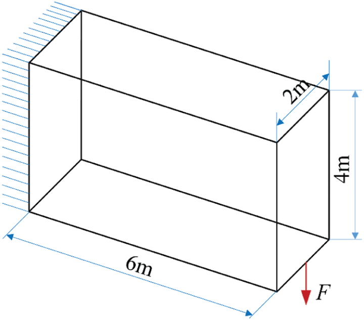
Fig. 10: Design domain, dimensions and boundary condition of a 3D cantilever

When the compliance is minimized subject to the total mass constraint, M¯T=7.2×103kg, Fig. 11 shows the optimized multi-material designs under various combinations of materials: (a) void, m1, m2 and m3; (b) void, m2 and m3; (c) void, m1 and m3; (d) void, m1 and m2. The corresponding compliances of the optimized multi-material designs are 4.01 Nm, 4.46 Nm, 4.06 Nm and 4.80 Nm, respectively. The compliance from the optimized design in Fig. 11a containing three solid materials is the minimum compared to other multi-material designs in Figs. 11b–11d, which only contain two solid materials. This also indicates that the performance of the multi-material design can be improved as more candidate materials are involved in optimization. Meanwhile, the proposed FPTO algorithm gives smooth interfaces between adjacent materials of the optimized 3D multi-material designs.

Next, the multi-material lightweight design is applied by specifying the displacement constraint at point A, uA≤0.6mm. Fig. 12 shows the optimized multi-material designs and the final masses under the various combinations of materials: (a) void, m1, m2 and m3; (b) void, m2 and m3; (c) void, m1 and m3; (d) void, m1 and m2. Compared with two-material designs in Figs. 12b–12d, the three-material design in Fig. 12a achieves the lowest mass to satisfy the specified displacement constraint.

Figure 11: 3D Multi-material designs for minimizing compliance under a mass constraint, M¯=7.2×103kg: (a) the optimized design using void, m1, m2 and m3, and its compliance is 4.01 Nm; (b) the optimized design using void, m2 and m3, and its compliance is 4.46 Nm; (c) the optimized design using void, m1 and m3, and its compliance is 4.06 Nm; (d) the optimized design using void, m1 and m2, and its compliance is 4.80 Nm

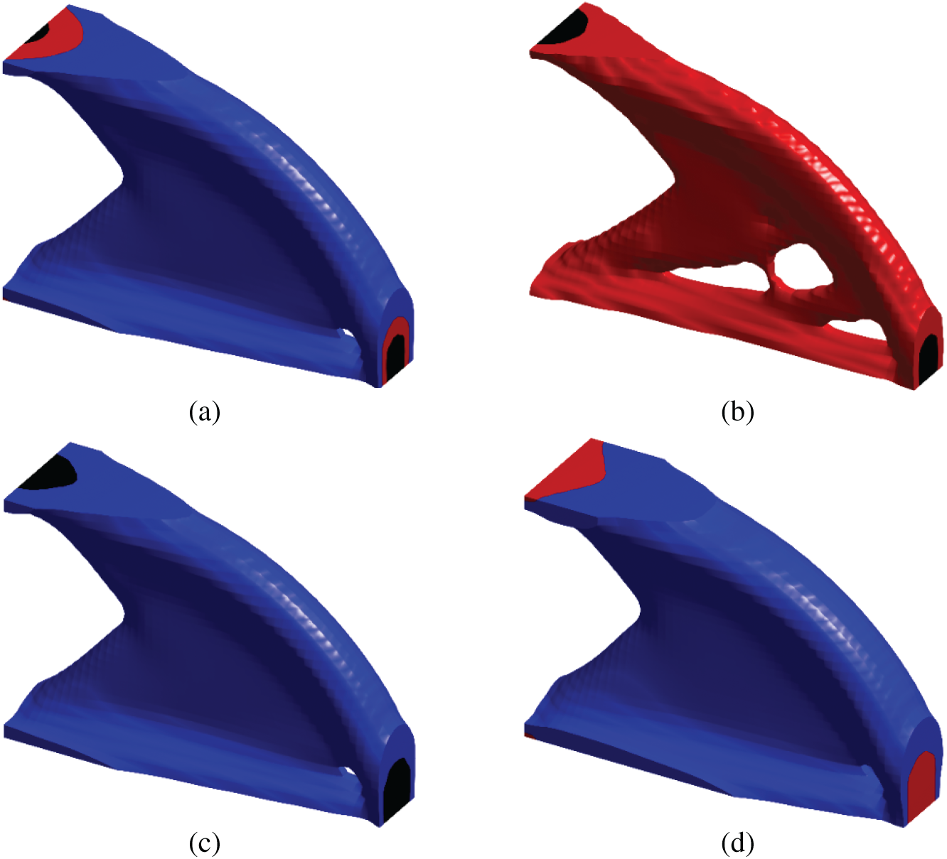
Figure 12: 3D multi-material designs for minimizing mass under a displacement constraint, uA≤0.6mm: (a) the optimized design using void, m1, m2 and m3, and the final mass is 3.768×103kg; (b) the optimized design using void, m2 and m3, and the final mass is 4.368×103kg; (c) the optimized design using void, m1 and m3, and the final mass is 3.792×103kg; (d) the optimized design using void, m1 and m2, and the final mass is 4.56×103kg

5  Conclusion

This paper proposed a new and simple multi-material topology optimization algorithm for minimizing compliance subject to a single mass constraint based on the FPTO method. Under the framework of the finite element analysis, the elemental normalized density is used as a single variable for designing structures composed of multiple materials without the increase of the computational burden. The ordered ersatz material model is proposed to interpolate the material property for the relaxed design variables linearly. Some 2D and 3D examples are presented to demonstrate the effectiveness of the proposed multi-material topology optimization algorithm and optimized multi-material designs are represented by the smooth interfaces between any two adjacent materials. Besides, the proposed algorithm can be extended to minimizing the total mass subject to single or multiple displacement constraints for a lightweight design of structures. Numerical results show that the multi-material designs could outperform the traditional solid/void designs, and this performance improvement increases when more candidate materials are involved in optimization.

Funding Statement: This work was supported by Hunan Provincial Innovation Foundation for Postgraduate (CX20190278), FJUT Scientific Research Foundation (GY-Z17015), and Open Fund of Fujian Key Laboratory of Automotive Electronics and Electric Drive (KF-X19001).

Conflicts of Interest: The authors declare that they have no conflicts of interest to report regarding the present study.

References

 1.  Bendsøe, M. P., Kikuchi, N. (1988). Generating optimal topologies in structural design using a homogenization method. Computer Methods in Applied Mechanics and Engineering, 71(2), 197–224. DOI 10.1016/0045-7825(88)90086-2. [Google Scholar] [CrossRef]

 2.  Suzuki, K., Kikuchi, N. (1991). A homogenization method for shape and topology optimization. Computer Methods in Applied Mechanics and Engineering, 93(3), 291–318. DOI 10.1016/0045-7825(91)90245-2. [Google Scholar] [CrossRef]

 3.  Nishiwaki, S., Frecker, M. I., Min, S., Kikuchi, N. (1998). Topology optimization of compliant mechanisms using the homogenization method. International Journal for Numerical Methods in Engineering, 42(3), 535–559. DOI 10.1002/(ISSN)1097-0207. [Google Scholar] [CrossRef]

 4.  Bendsøe, M. P. (1989). Optimal shape design as a material distribution problem. Structural Optimization, 1, 193–202. DOI 10.1007/BF01650949. [Google Scholar] [CrossRef]

 5.  Bendsøe, M. P., Sigmund, O. (2003). Topology optimization: Theory, methods and applications. Verlag, Berlin: Springer. [Google Scholar]

 6.  Sethian, J. A., Wiegmann, A. (2000). Structural boundary design via level set and immersed interface methods. Journal of Computational Physics, 163(2), 489–528. DOI 10.1006/jcph.2000.6581. [Google Scholar] [CrossRef]

 7.  Wang, M. Y., Wang, X., Guo, D. (2003). A level set method for structural topology optimization. Computer Methods in Applied Mechanics and Engineering, 192(1/2), 227–246. DOI 10.1016/S0045-7825(02)00559-5. [Google Scholar] [CrossRef]

 8.  Allaire, G., Jouve, F., Toader, A. M. (2004). Structural optimization using sensitivity analysis and a level-set method. Journal of Computational Physics, 194(1), 363–393. DOI 10.1016/j.jcp.2003.09.032. [Google Scholar] [CrossRef]

 9.  Querin, O. M., Steven, G. P., Xie, Y. M. (1998). Evolutionary structural optimization (ESO) using a bi-directional algorithm. Engineering Computations, 15, 1031–1048. DOI 10.1108/02644409810244129. [Google Scholar] [CrossRef]

10. Huang, X., Xie, Y. M. (2007). Convergent and mesh-independent solutions for the bi-directional evolutionary structural optimization method. Finite Elements in Analysis and Design, 43(14), 1039–1049. DOI 10.1016/j.finel.2007.06.006. [Google Scholar] [CrossRef]

11. Huang, X., Xie, Y. M. (2010). Evolutionary topology optimization of continuum structures: Methods and applications. John Wiley & Sons, Chichester. [Google Scholar]

12. Huang, X., Zuo, Y. H., Xie, Y. M. (2010). Evolutionary topological optimization of vibrating continuum structures for natural frequencies. Computers and Structures, 88, 357–364. DOI 10.1016/j.compstruc.2009.11.011. [Google Scholar] [CrossRef]

13. Sigmund, O., Torquato, S. (1997). Design of materials with extreme thermal expansion using a three-phase topology optimization method. Journal of the Mechanics & Physics of Solids, 45(6), 1037–1067. DOI 10.1016/S0022-5096(96)00114-7. [Google Scholar] [CrossRef]

14. Sigmund, O. (2001). Design of multiphysics actuators using topology optimization—Part II: Two-material structures. Computer Methods in Applied Mechanics and Engineering, 190, 6605–6627. DOI 10.1016/S0045-7825(01)00252-3. [Google Scholar] [CrossRef]

15. Gibiansky, L. V., Sigmund, O. (2000). Multiphase composites with extremal bulk modulus. Journal of the Mechanics & Physics of Solids, 48(3), 461–498. DOI 10.1016/S0022-5096(99)00043-5. [Google Scholar] [CrossRef]

16. Chu, S., Xiao, M., Gao, L., Li, H., Zhang, J. et al. (2019). Topology optimization of multi-material structures with graded interfaces. Computer Methods in Applied Mechanics and Engineering, 346, 1096–1117. DOI 10.1016/j.cma.2018.09.040. [Google Scholar] [CrossRef]

17. Jeong, S. H., Choi, D. H., Yoon, G. H. (2014). Separable stress interpolation scheme for stress-based topology optimization with multiple homogenous materials. Finite Elements in Analysis and Design, 82, 16–31. DOI 10.1016/j.finel.2013.12.003. [Google Scholar] [CrossRef]

18. Wang, M. Y., Wang, X. (2004). “Color” level sets: A multi-phase method for structural topology optimization with multiple materials. Computer Methods in Applied Mechanics and Engineering, 193, 469–496. DOI 10.1016/j.cma.2003.10.008. [Google Scholar] [CrossRef]

19. Guo, X., Zhang, W. S., Zhong, W. (2014). Stress-related topology optimization of continuum structures involving multi-phase materials. Computer Methods in Applied Mechanics and Engineering, 268, 632–655. DOI 10.1016/j.cma.2013.10.003. [Google Scholar] [CrossRef]

20. Huang, X., Xie, Y. M. (2009). Bi-directional evolutionary topology optimization of continuum structures with one or multiple materials. Computational Mechanics, 43(3), 393–401. DOI 10.1007/s00466-008-0312-0. [Google Scholar] [CrossRef]

21. Xu, B., Jiang, J. S., Xie, Y. M. (2015). Concurrent design of composite macrostructure and multi-phase material microstructure for minimum dynamic compliance. Composite Structures, 128, 221–233. DOI 10.1016/j.compstruct.2015.03.057. [Google Scholar] [CrossRef]

22. Da, D., Cui, X. Y., Long, K., Li, G. Y. (2017). Concurrent topological design of composite structures and the underlying multi-phase materials. Computers and Structures, 179, 1–14. DOI 10.1016/j.compstruc.2016.10.006. [Google Scholar] [CrossRef]

23. Xu, B., Huang, X., Zhou, S. W., Xie, Y. M. (2016). Concurrent topological design of composite thermoelastic macrostructure and microstructure with multi-phase material for maximum stiffness. Composite Structures, 150, 84–102. DOI 10.1016/j.compstruct.2016.04.038. [Google Scholar] [CrossRef]

24. Radman, A., Huang, X., Xie, Y. M. (2014). Topological design of microstructures of multi-phase materials for maximum stiffness or thermal conductivity. Computational Materials Science, 91, 266–273. DOI 10.1016/j.commatsci.2014.04.064. [Google Scholar] [CrossRef]

25. Da, D., Cui, X., Long, K., Cai, Y., Li, G. (2019). Multiscale concurrent topology optimization of structures and microscopic multi-phase materials for thermal conductivity. Engineering Computations, 36(1), 126–146. DOI 10.1108/EC-01-2018-0007. [Google Scholar] [CrossRef]

26. Zhang, W. S., Song, J., Zhou, J., Du, Z., Zhu, Y. et al. (2018). Topology optimization with multiple materials via moving morphable component (MMC) method. International Journal for Numerical Methods in Engineering, 113, 1653–1675. DOI 10.1002/nme.5714. [Google Scholar] [CrossRef]

27. Wang, M., Zhou, S. (2004). Phase field: A variational method for structural topology optimization. Computer Modeling in Engineering and Science, 6(6), 547–566 DOI 10.1115/DETC2004-57637. [Google Scholar] [CrossRef]

28. Tavakoli, R., Mohseni, S. (2013). Alternating active-phase algorithm for multimaterial topology optimization problems: A 115-line MATLAB implementation. Structural and Multidisciplinary Optimization, 49(4), 621–642. DOI 10.1007/s00158-013-0999-1. [Google Scholar] [CrossRef]

29. Park, J., Sutradhar, A. (2015). A multi-resolution method for 3D multi-material topology optimization. Computer Methods in Applied Mechanics and Engineering, 285, 571–586. DOI 10.1016/j.cma.2014.10.011. [Google Scholar] [CrossRef]

30. Wang, N. F., Hu, K., Zhang, X. M. (2017). Hierarchical optimization for topology design of multi-material compliant mechanisms. Engineering Optimization, 49(12), 2013–2035. DOI 10.1080/0305215X.2016.1277062. [Google Scholar] [CrossRef]

31. Wei, P., Wang, M. Y. (2009). Piecewise constant level set method for structural topology optimization. International Journal for Numerical Methods in Engineering, 78, 379–402. DOI 10.1002/nme.2478. [Google Scholar] [CrossRef]

32. Luo, Z., Tong, L., Luo, J., Wei, P., Wang, M. Y. (2009). Design of piezoelectric actuators using a multiphase level set method of piecewise constants. Journal of Computational Physics, 228, 2643–2659. DOI 10.1016/j.jcp.2008.12.019. [Google Scholar] [CrossRef]

33. Wang, Y., Luo, Z., Kang, Z., Zhang, N. (2015). A multi-material level set-based topology and shape optimization method. Computer Methods in Applied Mechanics and Engineering, 283, 1570–1586. DOI 10.1016/j.cma.2014.11.002. [Google Scholar] [CrossRef]

34. Yin, L., Ananthasuresh, G. K. (2001). Topology optimization of compliant mechanisms with multiple materials using a peak function material interpolation scheme. Structural and Multidisciplinary Optimization, 23, 49–62. DOI 10.1007/s00158-001-0165-z. [Google Scholar] [CrossRef]

35. Gao, T., Zhang, W. (2011). A mass constraint formulation for structural topology optimization with multiphase materials. International Journal for Numerical Methods in Engineering, 88, 774–796. DOI 10.1002/nme.3197. [Google Scholar] [CrossRef]

36. Gao, T., Xu, P., Zhang, W. (2016). Topology optimization of thermos-elastic structures with multiple materials under mass constraint. Computers and Structures, 173, 150–160. DOI 10.1016/j.compstruc.2016.06.002. [Google Scholar] [CrossRef]

37. Zuo, W., Saitou, K. (2017). Multi-material topology optimization using ordered SIMP interpolation. Structural and Multidisciplinary Optimization, 55, 477–491. DOI 10.1007/s00158-016-1513-3. [Google Scholar] [CrossRef]

38. Yang, X. T., Li, M. (2018). Discrete multi-material topology optimization under total mass constraint. Computer-Aided Design, 102, 182–192. DOI 10.1016/j.cad.2018.04.023. [Google Scholar] [CrossRef]

39. Huang, X. (2020). Smooth topological design of structures using the floating projection. Engineering Structures, 208, 110330. DOI 10.1016/j.engstruct.2020.110330. [Google Scholar] [CrossRef]

40. Huang, X. (2021). On smooth or 0/1 designs of the fixed-mesh element-based topology optimization. Advances in Engineering Software, 151, 102942. DOI 10.1016/j.advengsoft.2020.102942. [Google Scholar] [CrossRef]

41. Sigmund, O., Petersson, J. (1998). Numerical instabilities in topology optimization: A survey on procedures dealing with checkerboards, mesh-dependencies and local minima. Structural Optimization, 16(1), 68–75. DOI 10.1007/BF01214002. [Google Scholar] [CrossRef]

This work is licensed under a Creative Commons Attribution 4.0 International License, which permits unrestricted use, distribution, and reproduction in any medium, provided the original work is properly cited.