Computer Modeling in Engineering & Sciences

DOI: 10.32604/cmes.2021.016269

ARTICLE

A Computational Study on Lateral Flight Stability of the Cranefly in Hover

Na Xu1, Shuaizhi Zhou1, Chunchen Zhang1 and Xiaolei Mou2,*

1School of Electromechanical and Automotive Engineering, Yantai University, Yantai, 264005, China
2School of Civil Engineering, Yantai University, Yantai, 264005, China
*Corresponding Author: Xiaolei Mou. Email: xiaoleimou@126.com
Received: 22 February 2021; Accepted: 07 May 2021

1  Introduction

Since the insects flying in nature are disturbed by the surroundings all the time, the problems that how the insects change the flight attitude with the influence of external disturbances, how they maintain a stable flight attitude and speed, and how they achieve the inspired performances, such as an abrupt stop, turn, fast acceleration, should be investigated. To reveal the flight dynamic stability and control mechanism of insects, extensive studies on these above problems have been conducted in recent decades, which are available in the literature reviews [1,2]. Considering that the flight dynamics of a flapping-wing flier is inherently complex, and only the dynamic stability is thoroughly researched can the control problem be adequately understood, many investigations mainly focused on dynamic flight stability to examine the stability derivatives, dynamic modal structure and quantitative stability properties [3–13].

In the above investigations [3–13], with the averaged model widely employed, the flapping-wing fliers are approximately treated as rigid bodies with six degrees of freedom (6-DOF), the equations of motion of which are similar to the conventional aircraft; then using the linear theory, the disturbed flight in the longitudinal and lateral direction are treated separately after decoupling, and in turn, the stability of the flapping-wing systems could be checked by techniques of eigenvalue and eigenvector analyses. The disturbed flight includes longitudinal and lateral motion, and only both longitudinal and lateral dynamics are figured out can the stability characteristics of insects be known.

During the past two decades, many research work, employing different aerodynamic models, the CFD method or the quasi-steady model, have been concentrated on the longitudinal dynamic stability [4–6,9,10,12,13] for several hovering insects (e.g., bumblebee, hoverfly, dronefly, cranefly, fruitfly, stalk-eyed fly, hawkmoth and mosquito) and the literatures reported that three longitudinal natural modes (two stable subsidence modes and one unstable oscillatory mode) in hover were identified, thus the hovering flight in longitudinal was unstable. In addition, the conclusions of longitudinal dynamic stability mentioned above were consistent, although the mass of research objects ranged from 1 to 1648 mg and wing-beat frequency from 26 to 800 Hz [2,13,14]. With the wider range of weight and wing-beat frequency, the longitudinal dynamic stability characteristics mentioned above may represent those of the majority of insects.

Researches on lateral dynamic stability of several hovering insects were carried out gradually, and all the literatures pointed out the lateral disturbed flight was composed of three natural modes of motion. However, the modal structure of lateral motion for different hovering insects is not exactly the same. The works in Zhang et al. [8] and Xu et al. [11,15] reported that the lateral motion of hovering insects (dronefly, hoverfly and bumblebee) was unstable, due to the divergence mode; and works in Faruque et al. [7], Cheng et al. [9] and Kim et al. [12] showed that all the natural modes of hovering insects (fruitfly, hawkmoth, stalk-eyed fly and bumblebee) in lateral were stable. Hereafter, the study on the lateral dynamic stability of hovering honeybee [16] pointed that the lateral disturbed motion consisted of a nearly neutrally stable oscillatory mode and two stable subsidence modes, hence the flight was neutrally stable. The difference in the modal structure of lateral motion could be attributed to the different sign of the derivative of roll moment vs. sideslip velocity [11,12,16] (hereafter called as roll-moment/sideslip-velocity derivative). Contributions on the generation of the roll-moment/sideslip-velocity derivative included two flow effects: ‘changing-relative-velocity’ effect and ‘changing-LEV-axial-velocity’ effect (hereafter abbreviated as CRV-effect and CLV-effect), and the relative sizes of which determined the sign of the derivative [11,15,16].

As noted above, the researches on longitudinal dynamics in hover cover many kinds of insects, additionally with various aspect ratios (AR, the ratio of wing length to mean chord length), and the longitudinal dynamic stability characteristics mentioned are similar. However, the roll-moment/sideslip-velocity derivative could be affected by certain parameters, e.g., the location of the CG (the center of gravity), the stroke plane angle [15,16]. In addition, the recent study [17] pointed out the wing-wing interaction had influence on the roll-moment/sideslip-velocity derivative and the contralateral wing stabilized the hovering hawkmoth in lateral. In other words, the lateral stability, which may have different modal structure, is not as robust as that of longitudinal. Furthermore, the insects considered in the studies of lateral dynamic stability are mostly with moderate aspect ratios (AR = 2–4), excluding the insects with a relatively large aspect ratio. Researches have showed that the change in AR have the influence on the flow structure of the rotating and flapping wings [18–20] and hence the aerodynamic forces acting on the wings. This situation may have impact on the aerodynamics of insects with a relatively large aspect ratio in disturbed flight, especially the roll-moment/sideslip-velocity derivative that can result in the lateral stability changing. For some insects, even without the wing-wing interaction, the CLV-effect may decrease due to a relatively large aspect ratio, and the relative size of roll moments produced by the two flow effects involved above which have opposite signs accordingly changed, and hence the negative roll-moment/sideslip-velocity derivative and the flight stability would become different. Recently, Liu et al. [13] have discussed the dynamic stability of mosquitoes in hover of which the aspect ratio is indeed relatively large (AR = 5), and the results showed that the dynamic modal structure of mosquitoes is similar to that of other insects, such as bumblebee and hoverfly. However, the mosquitos used different mechanisms to generate aerodynamic forces due to the rather short stroke amplitude [14], while much more insects considered above mainly use the same delayed-stall mechanism. Among the insects studied above, the cranefly has a relatively large aspect ratio (AR = 5.5) and also use the delayed-stall mechanism. From the foregoing discussion, it is meaningful to investigate the lateral dynamic stability of hovering cranefly to see whether or not it has similar dimensionless stability derivatives and dynamic modal structure with other insects.

In this paper, taking a model cranefly in hover as the research object, numerical research on its lateral dynamic stability is conducted. First, the incompressible Navier-Stokes equations are solved to acquire the stability derivatives, and then the eigenvalues and eigenvectors of the system matrix are derived to characterize the lateral dynamics. The analysis results verify the previous hypothesis: the roll-moment/sideslip-velocity derivative of the model cranefly is negative and a different dynamic modal structure from most other insects is identified.

2  Materials and Methods

2.1 Morphology and Kinematics

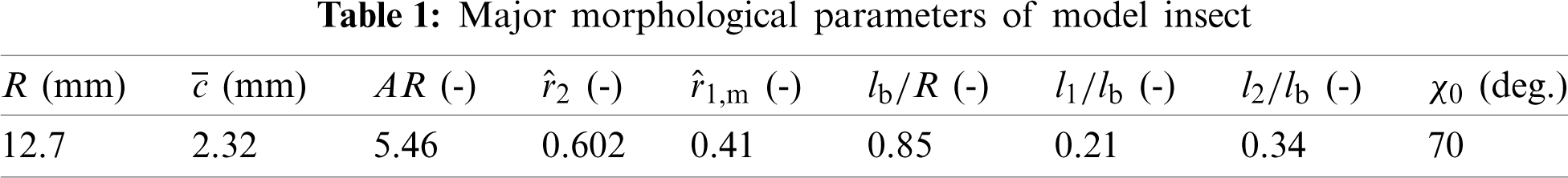
In this study, the cranefly Tipula obsoleta is conducted as the research target based on measurement data [21], the total weight of the cranefly m=11.4 mg and the mass fraction of one wing of the total weight m^w=2.14%. The major morphological parameters of wings and body are detailed in Tab. 1. For wings, R denotes the wing length, c¯ denotes the mean chord of one wing, the aspect ratio of one wing AR equals to R/c¯, the radius r^2 represents the ratio of the second moment of wing area to wing length, and r^1,m is the distance between wing root and its center of mass. For the body, lb denotes the body length, l1 is the distance from the wing-root pivot to CG, l2 is the radius of gyration for the moment of inertia about the wing-root axis and χ0 is free body angle [21,22].

In order to describe the definitions of the wing and body kinematics, two coordinate systems are introduced here: a right-handed body-fixed frame (obxbybzb) and a wing-fixed frame (owxwywzw). The body-fixed frame is located at the CG with origin ob. Assuming the insect bilateral symmetry, the xb–zb plane is arranged in the longitudinal symmetrical plane and yb-axis points to the right. The model cranefly considered here is hovering, thus the velocity of the body is zero and body angle χ between body axis (longitudinal blue dash-dot line) and the horizontal (Fig. 1A) determines its orientation.

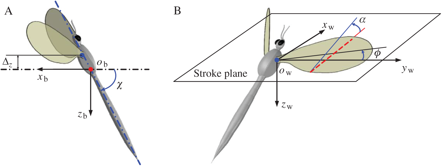
Figure 1: Schematics of the kinematics of model insect (A) the right-handed body-fixed frame, (B) the wing-fixed frame

The origin of the wing-fixed frame ow is located at the wing pivot point (blue point in Fig. 1B). The xw- and yw-axes are arranged in the stroke plane with yw-axis pointing to the side of the insect (Fig. 1B). Based on the experimental measurements [22], the wing flaps within the stroke plane when neglecting the motion of wingtip deviating from the stroke plane. Hence adopting the convention in previous studies [4,11,23], the wing’s motion here is defined by two angles ϕ and α, see Fig. 1B. ϕ is the stroke positional angle, defining the translation rotation around zw-axis and α is the angle of attack, defining the rotation around the wing-span axis (yw-axis).

When the wing flaps to its extreme position, the stroke positional angle ϕ reaches the minimum and maximum values, recorded as ϕmin and ϕmax, respectively. The stroke amplitude is denoted by the letter Φ (=ϕmax−ϕmin) and the mean stroke angle by the letter ϕ¯(=(ϕmax+ϕmin)/2). The angle of attack (α) keeps unchanged in mid-downstroke and mid-upstroke while it varies with time when the wing flips close to the extreme position. The unchanged value of α in mid-downstroke and mid-upstroke herein are notated with αd and αu, respectively, and taken the supination at k-th stroke cycle, the variation of ϕ and α are represented as the following harmonic functions:

{ϕ=ϕ¯+Φ2cos⁡(2πft)α=αd+180∘−αd−αuΔtr[(t−t1)−Δtr2πsin2π(t−t1)Δtr],t1≤t≤t1+Δtrt1=kT−0.5T−0.5Δtr (1)

where f denotes the flapping frequency, t1 the time when the supination starts, Δtr the duration of wing’s supination and T (=2Φr^2R/c¯) denotes the flapping period. The time behavior of α in pronation is similar to that in supination. According to Eq. (1), it is certain that kinematic parameters ϕ¯, Φ, f, αd, αu and Δtr should be determined to describe the flapping motion. Considering that the angles ϕ and α are measured with respect to the stroke plane, the stroke plane angle β representing the inclination of the plane to the horizontal also needs to be given. The angle that describes the motion deviating from the stroke plane herein is ignored.

All the kinematic parameters needed to describe the motions of body and wing are detailed in Tab. 2 and determined from experimental data by Ellington [22], excluding ϕ¯, αd and αu. These three angles will be calculated by finding the equilibrium flight conditions (see Section 2.4), due to the difficulty in accurately measuring.

2.2 Equations of Motion

Referring to the earlier studies [3,4,8], the averaged model is applied in the present study. Provided the model insect presents a relatively high wingbeat frequency, it is assumed that the flapping flier can be treated like a 6-DOF rigid body (three in translation and three in rotation) and use the mean aerodynamic forces and moments through the flapping period to represent the role of wings in aerodynamics. Therefore, the motions of model insect are expressed by the equations of motion of rigid body, commonly used for the airplane or helicopter.

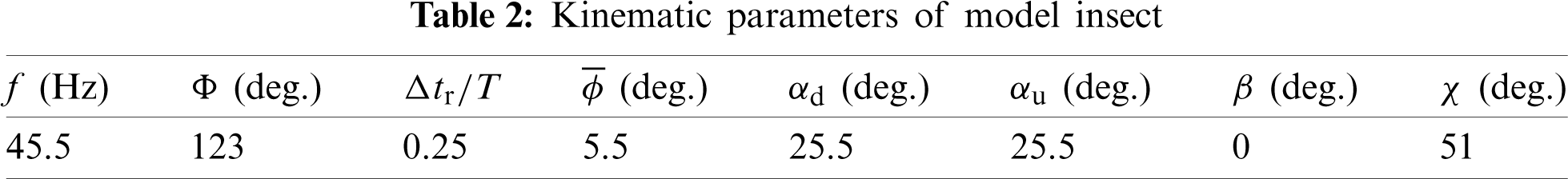
For the convenience of describing the movements of model insect, the right-handed frame of reference (obxbybzb) is used (see Fig. 1A); at the equilibrium flight, xb–zb plane is located in the longitudinal plane of symmetry with xb-axis pointing to the front and yb-axis faces towards the right (Fig. 2). Similar to the handling of an airplane, the motions of the insect’s body are assumed to slightly deviate from a steady, symmetric reference flight condition and all flight parameters in the equations can be written in the form of reference value plus disturbance. Using the small-disturbance linearization theory, the lateral equations of motion can be considered in isolation from the longitudinal ones. The variable statements involved in the lateral motion are listed as follows: the motion variable v denotes the velocity in the yb direction; the angular velocities p is called the roll velocity around the xb-axis and r called the yaw velocity around the zb-axis; and the roll angle γ defines the inclination of yb-axis against the horizontal (Fig. 2).

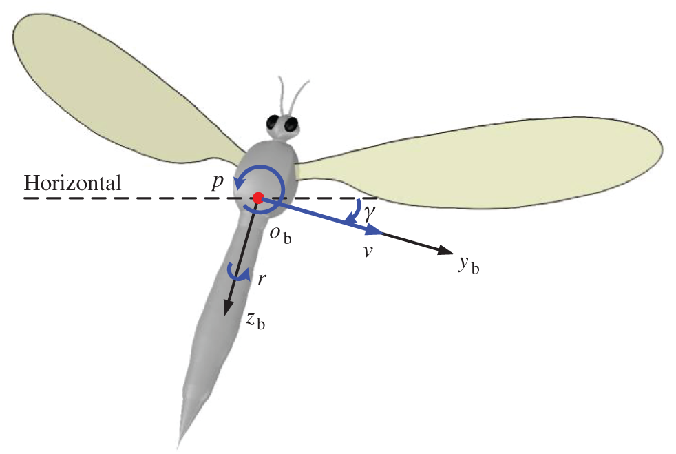
Figure 2: Definition of the lateral state variables

For the convenience in analyzing, the components of average aerodynamic forces through the flapping period are recorded as X, Y and Z (forward, lateral and vertical force), respectively; and the components of average moments about the CG be L, M and N (roll, pitch and yaw moment), respectively. At hovering equilibrium flight, Y=L=N=0 and v=p=r=γ=0 (γ=0 implies that the yb-axis lies in the horizontal plane at the equilibrium reference condition), and the linearized lateral equations of motion are:

[δv˙+δp˙+δr˙+δγ˙]=A[δv+δp+δr+δγ] (2)

where the matrix A is the stability system matrix, the prefix δ represents the small perturbation value, the overdot “·” represents differentiation with respect to time:

A=[ Yv+m+Yp+m+Yr+m+g+Iz+Lv++Ixz+Nv+Ix+Iz+−Ixz+2Iz+Lp++Ixz+Np+Ix+Iz+−Ixz+2Iz+Lr++Ixz+Nr+Ix+Iz+−Ixz+20Ixz+Lv++IxNv+Ix+Iz+−Ixz+2Ixz+Lp++Ix+Np+Ix+Iz+−Ixz+2Ixz+Lr++Ix+Nr+Ix+Iz+−Ixz+200100 ] (3)

In the matrix A, the symbols (Yv, Lv, Nv), (Yp, Lp, Np), (Yr, Lr, Nr) denote the stability derivatives of the aerodynamic forces (Y, L and N) with respect to the state variables (v, p and r). The superscript “+” herein denotes the dimensionless quantity; using the mean chord length c¯ as the characteristic length, the flapping period tw (=1/f) as the characteristic time and the mean flapping velocity U (=2Φr^2Rf) as the characteristic velocity, the dimensionless forms are: aerodynamic force Y+=Y/0.5ρU2St (hereafter St represents the total area of two wings), aerodynamic moments L+=L/0.5ρU2Stc¯, N+=N/0.5ρU2Stc¯; translational velocity v+=v/U, angular velocity p+=ptw, r+=rtw; total mass m+=m/0.5ρUSttw; the acceleration of gravity g+=gtw/U; time t+=t/tw; the moments of inertia Ix+=Ix/0.5ρU2Stc¯tw2, Iz+=Iz/0.5ρU2Stc¯tw2, the product of inertia Ixz+=Ixz/0.5ρU2Stc¯tw2.

The moments of inertia about xb and zb-axes and product of inertia (Ix, Iz and Ixz) of the model cranefly in this study are estimated using the method similar to that of the earlier study [8]. For the model cranefly at hovering, Ix=7.346×10−11 kgm2, Iz=5.509×10−11 kgm2, Ixz=−4.221×10−11 kgm2. Now, in order to specify the system matrix A, only the stability derivatives need to be determined.

2.3 Flow Computation and Grid Resolution Test

By solving the Navier–Stokes (N-S) equations, the equilibrium flight condition can be obtained, and hence the determination of stability derivatives. In this study, the identical numerical calculating method which Sun et al. [23] had given the detailed description in their work is adopted for simulation and based on the artificial compressibility approach [24]. The earlier research result [25] showed that the corrugation and deformation of wings in the flapping have little effects on aerodynamic forces, and thus the wing of model insect can be dealt with as a rigid plate by neglecting the corrugation and deformation. By comparison with wings, the body has very low velocity near hovering and thus the aerodynamic forces and moments generated by the body are negligible; besides, the aerodynamic interference between the wings and body is so weak that it can be neglected, as well as the interference between the right and left wings [26]. Thus, the flow around the right and left wing can be calculated separately.

In this study, the planform of wing model used here is taken from the scanned image of the real wing [21] (Fig. 3, the solid line with an arrow indicates the pitching rotation axis). The numerical calculation program used here has been validated and used many times in previous studies (e.g., [8,11,23]). Reynolds number (Re) is defined as Re=Uc¯/ν, where the kinematic viscosity ν is 1.44×10−5 m2s−1 for the air and based on the morphology and kinematics data given above Re for the model cranefly is approximately 240.

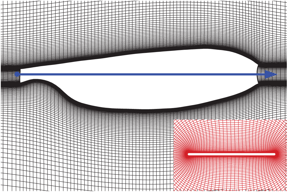
Figure 3: The planform of the wing and portions of the grid. The inset is the sectional plane at the radius of gyration (r^2)

In order to make sure that the flow simulations are grid independent, three grids are used herein to conduct the grid resolution test before the simulations. The size of Grid 1 is 25 × 27 × 34 (in the circumferential direction, the radial direction and the spanwise direction, respectively) with the first layer spacing of 0.004c¯. Grid 2 and Grid 3 have dimensions 50 × 53 × 68 and 100 × 105 × 135 with the first layer spacing of 0.002c¯ and 0.001c¯, respectively. The computational domain size of these three grids is 20c¯ away from the wing surface in the radial direction and 7c¯ in the spanwise direction. The lift and drag coefficients over a single flapping cycle calculated by these three grids are showed in Fig. 4. It can be found from Fig. 4 that the first grid refinement makes some differences in the aerodynamic force coefficients and almost no differences for the second refinement. Based on the test results, Grid 3 is chosen for the flow simulations.

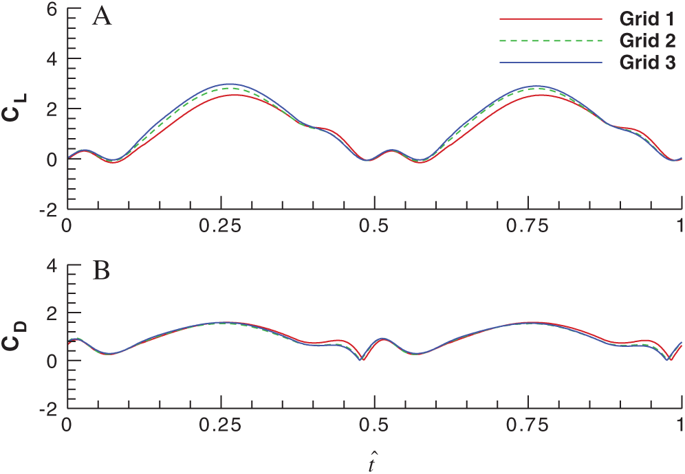
Figure 4: Effects of grid density on the lift and drag coefficients over a single flapping cycle (A) for the lift coefficient and (B) for the drag coefficient

2.4 Calculation of the Stability Derivatives

As aforementioned, ϕ¯, αd and αu will be calculated by satisfying the equilibrium conditions: the mean vertical force of the wings equals the weight of insect (Ze=mg); the mean forward force and pitch moment equal to zero (Xe=0, Me=0). Considering the difficulty in accurately measuring wing kinematics, if the kinematics parameters of wings used for force balance are all measured data, the equilibrium conditions could not be obtained. Meanwhile, there are three equations to satisfy in equilibrium conditions, and the variation in ϕ¯ is a sensitive effect on aerodynamic moments, and the measurement errors of αd and αu are relatively large [27], thus these three parameters ϕ¯, αd and αu are obtained by satisfying the equilibrium flight conditions, instead of from experimental data. The solution process is briefly shown in Fig. 5, and the corresponding ϕ¯, αd and αu to the equilibrium flight are listed in Tab. 2.

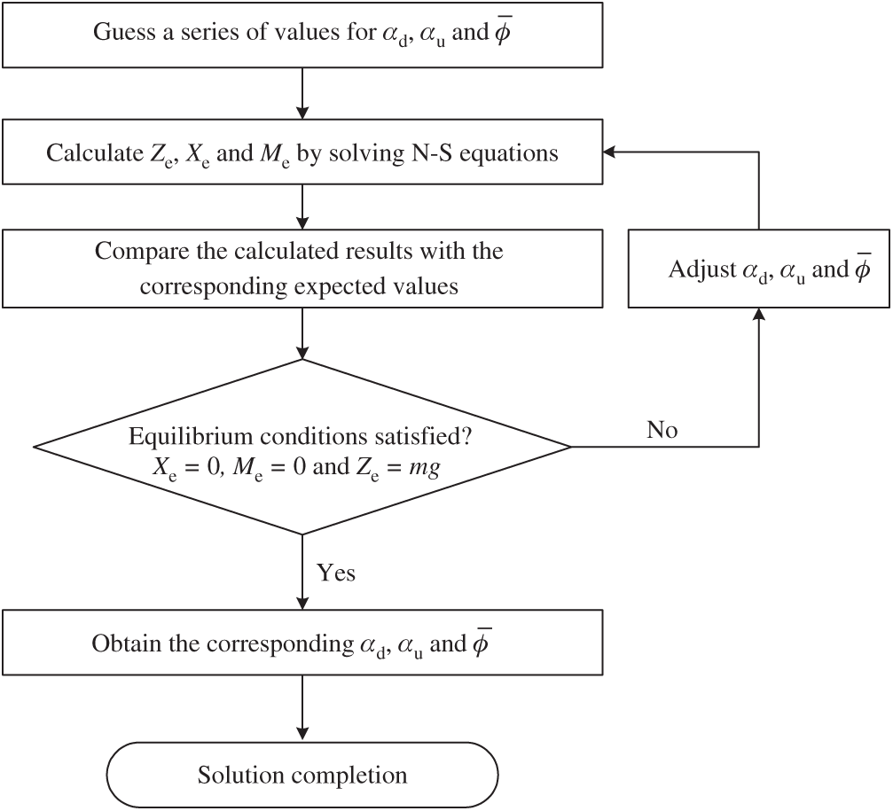
Figure 5: The solution process of equilibrium conditions achievements

Once the equilibrium flight is determined, we can use it as the reference flight state to acquire the stability derivatives. Adopting the same method as taken in the previous studies [8,11], three series of flow computations are conducted. For each series, only one of the body velocities varies near zero whilst the others keep the reference values unchanged. Take the v-series as an example, the lateral translational velocity v is varied whilst p=r=γ=0, and the varying wing-beat cycle average forces and moments are calculated; then the curves that represent the variation of average forces and moments with changes in the state variable v are fitted. The stability derivatives are derived from the local tangents of the fitted curves in the equilibrium state. By definition, the stability derivatives are partial derivatives, and hence represent the rates of change of forces and moments when the corresponding body velocity is varied. The p and r-series stability derivatives can be obtained by the same operation.

Once the derivatives are calculated, all the data needed in the system matrix A in Eq. (3) are determined. Adopting the same eigenvalues and eigenvectors analysis method in previous studies [4,8,11], the flight stability characteristics of the system are acquired from the linear small disturbance equations.

3  Results and Discussion

3.1 Stability Derivatives

As described above, on the basis of the equilibrium flight of model cranefly, the body velocities v, p and r vary around zero respectively and the corresponding aerodynamic forces and moments are obtained, which are shown in Fig. 6. Y+, L+ and N+, by definition, are the dimensionless quantities. The variations of aerodynamic forces and moments with body velocities for model cranefly in Fig. 6 show that, for state variables in the range of −0.15 and 0.15, the aerodynamic forces and moments vary approximately linearly with the body velocities, which indicates that the theory of small-disturbance linearization is applicable for this range. The lateral stability derivatives of hovering model cranefly, given by the slopes of the curves at the origin in Fig. 6, are listed in Tab. 3.

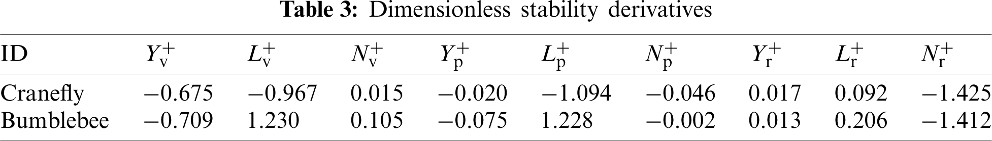
According to the results of Tab. 3, the lateral stability derivatives Yv+, Lp+ and Nr+ are negative and have large values whilst those of Nv+, Yp+, Np+, Yr+ and Lr+ are comparatively small. The mainly stability derivatives, Yv+, Lp+ and Nr+, of cranefly resemble those of dronefly [8], bumblebee [11] and hoverfly [15] investigated in the previous literature. The relatively large negative values of Yv+, Lp+ and Nr+ indicate that the body motions mainly produce the corresponding large damping. More specifically, the lateral translational motion (v+) generates a lateral force opposite to the direction of the translation, and the roll (p+) and yaw (r+) motion generate a large moment in the direction opposite to the rotation. As expected, Lv+ (roll moment induced by the lateral translation) of cranefly is negative, presenting an opposite sign to those of dronefly [8], bumblebee [11] and hoverfly [15]. The negative sign of Lv+ describes the fact that the roll moment induced by the lateral translational motion (v+) causes the insect to tilt toward the opposite direction of translation, and makes the lateral dynamic stability of model cranefly different from those of other insects above. Here, for comparative purposes, the data of bumblebee extracted from the literature [11] are also given in Tab. 3.

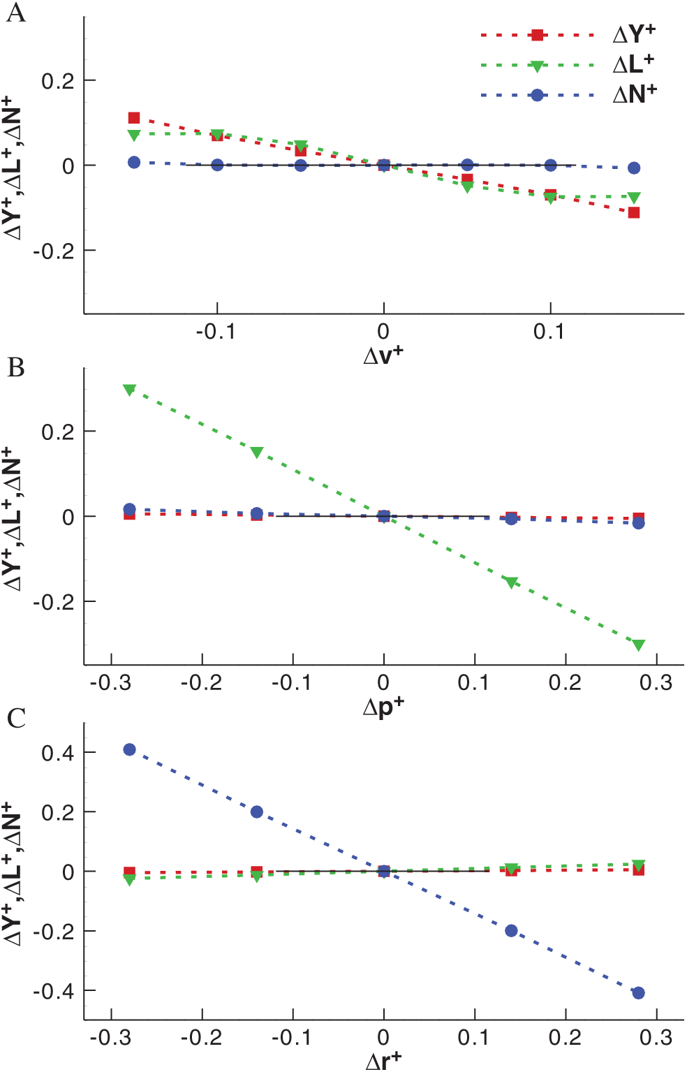
Figure 6: The variations of aerodynamic forces and moments with body velocities for model cranefly (A) for the v-series, (B) for the p-series and (C) for the r-series

3.2 Generation Mechanism of Stability Derivatives

As stated earlier, the generation of the mainly stability derivatives, Yv+, Lp+ and Nr+, of cranefly can be attributed to the damping mechanism that is similar to other insects. Here we focus on the negative derivative Lv+, the significant difference between the model cranefly and the other insects involved above. The previous studies [11,16] of lateral dynamic stability of insects have revealed that when the insect moves laterally (v+), the aerodynamic forces of flapping wings will be affected by the CRV-effect and CLV-effect, and the mechanism of these two effects is summarized here. The insect sees a lateral wind when moving laterally (v+), and the lateral wind can be decomposed into two components in the chordwise and spanwise direction, which are herein denoted by vr+ (=v+sin⁡ϕ) and va+ (=v+cos⁡ϕ), respectively. The chordwise component of lateral wind changes the relative velocity of flapping wings, causing the CRV-effect. It increases or decreases the relative velocity of flapping wings by |v+sin⁡ϕ|, and the change of right and left wing are opposite and have different signs in different stages of the flapping period; this leads to a roughly opposite change in aerodynamic forces on the two contralateral wings. Meanwhile, the lateral wind in spanwise direction changes the axial velocity of LEV on flapping wings by v+cos⁡ϕ, causing the CLV-effect. During the lateral translation, one wing always sees a spanwise flow from the wing base to tip and the other from tip to base, making the axial velocity increase on the former and decrease on the latter, and hence, the concentration of LEV on two wings are different. Due to the more concentrated vortex on one wing, a larger suction pressure above the wing is produced and thus gives a higher lift, and the opposite situation happens with the other wing; this also leads to the difference in aerodynamic forces of two wings. Here takes moving to the right as an example, the CRV-effect produces a net lateral force in the opposite direction of translation (v+) and the net lateral force induces a roll moment around the CG. Since the wing base lies above CG, the arm of lateral force is approximate as the vertical distance between the above two points (Δz) (Fig. 1), the roll moment induced by the lateral force makes a negative contribution to Lv+, and moreover, the negative contribution of the CRV-effect will augment with the increasing vertical distance. However, the CLV-effect produces a force couple, the roll moment of which makes a positive contribution to Lv+. For bumblebee [11] and hoverfly [16], the positive contribution of CLV-effect is greater than the negative counterpart of CRV-effect. Thus a positive Lv+ is obtained.

To illuminate the reason why the derivative Lv+ of model cranefly is opposite to that of model bumblebee in reference [11], the results of these two model insects are compared, and two symbols ΔYw+ and ΔZw+ are introduced. Yw and Zw are the components of aerodynamic forces produced by flapping wings, lateral force along the yb-axis and vertical force along the zb-axis, respectively; the prefix ‘Δ’ represents the difference between the disturbance motion and the corresponding equilibrium flight and the subscript ‘+’ represents the form of dimensionless force coefficients. The time-variation of ΔYw+ and ΔZw+ over a single flapping cycle when insects moving to the right with dimensionless velocity v+=0.15 are showed in Fig. 7 (the data of model bumblebee is extracted from reference [11], t^ is the dimensionless time). From Figs. 7A1 and 7B1, it can be seen that, under the lateral wind, the variation in ΔYw+ on the wings of cranefly is identical with that of bumblebee [11], and ΔYw+ for each wing are negative over a single flapping cycle, making a negative cycle averaged lateral force ΔY+. Although the variation tendency of ΔZw+ for cranefly and bumblebee [11] are the same: ΔZw+ of the right and left wing basically have a different sign in the whole wingbeat cycle and this produces a force couple around the roll axis, namely cycle averaged roll moment ΔLLEV+. However, there are indeed some differences in the magnitude of ΔZw+ between the model cranefly and bumblebee. For bumblebee in Fig. 7B2, during the downstroke, the magnitude of ΔZw+ in the first part (t^≈0−0.25, the pale blue region) is much smaller than that in the latter part (t^≈0.25−0.5, the lavender region). Thus the net vertical force on the left and right wing points upward and downward, respectively, as depicted in Fig. 8B, producing a force couple that makes the insect incline towards the translational direction, and the same is true for the upstroke. Hence, the net cycle averaged roll moment is positive [11]. Whereas, for cranefly in Fig. 7A2, during the downstroke or upstroke, the difference in the magnitude of ΔZw+ between the first part (t^≈0−0.25, the pale blue region or t^≈0.5−0.75) and the latter part (t^≈0.25−0.5, the lavender region or t^≈0.75−1) is relatively small. Take the downstroke for an example, there are few differences between the negative roll moment induced by the force couple in the first part (the pale blue) and the positive counterpart in the latter part (the lavender), as depicted in Fig. 8A. The same is true for the upstroke. Thus, the net cycle averaged roll moment induced by the force couple tends to be very small, which indicates that the CLV-effect might be weakened for model cranefly, comparing with that of model bumblebee. It can be seen from the spanwise vorticity plots of the wings at three instants during the flapping cycle showing in Fig. 9. Unlike the vorticity plots of bumblebee depicted in Fig. 8 in reference [11], it seems like there is little difference between the LEV on the left wing and that on the right wing, indicating the comparatively weak CLV-effect for the model cranefly.

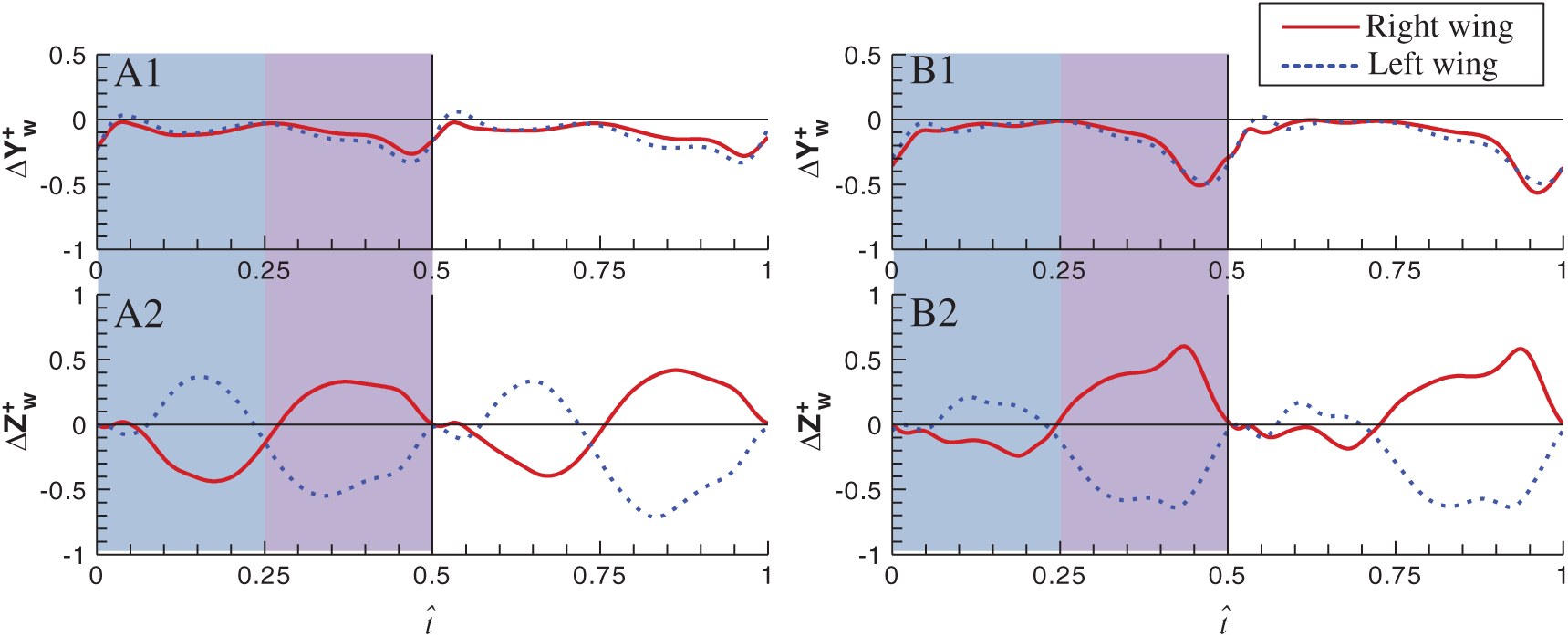
Figure 7: Time-variation of ΔYw+ and ΔZw+ at v+=0.15 over a single flapping cycle for the model cranefly and bumblebee (A for cranefly, B for bumblebee [11]; the red solid lines for right wings and the blue dashed lines for left wings). The first and latter parts of downstroke are indicated by the pale blue region and lavender region, respectively

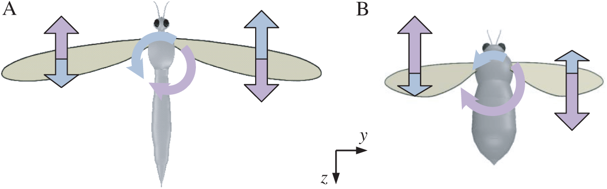
Figure 8: Schematics of roll moments produced by the force couple during the downstroke for model cranefly and bumblebee (A) for cranefly, (B) for bumblebee; the pale blue for the first part of the downstroke and the lavender for the latter part of the downstroke

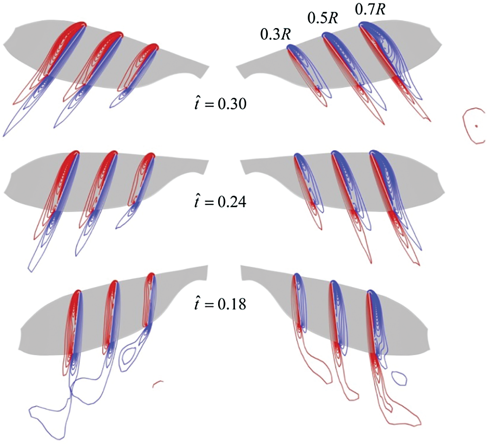
Figure 9: Spanwise vorticity plots at wing sections (0.3R, 0.5R, 0.7R from wing root, respectively) when the insect moves to the right at v+=0.15. The red and blue lines indicate the positive and negative vorticity, respectively. The magnitude of the nondimensional vorticity at the outer contour is 2 and the interval is 2

Next, the CRV-effect and CLV-effect of model cranefly and those of model bumblebee [11] will be quantitatively compared. Still take insects move to the right at v+=0.15 as an example, the cycle averaged lateral force (ΔY+), the dimensionless vertical distance (Δz+), the cycle averaged roll moment of the lateral force (ΔLRV+, ΔLRV+=Δz+×ΔY+) and of the couple (ΔLLEV+), and the total roll moment (ΔL+, ΔL+=ΔLRV++ΔLLEV+) are listed in Tab. 4 (the related data of bumblebee is extracted from reference [11]). Comparing two sets of data in Tab. 4, the values of Δz+ and ΔY+ of model cranefly are equivalent to those of model bumblebee, thus the negative ΔLRV+ of cranefly and that of bumblebee are about the same. However, the roll moment induced by the CLV-effect (ΔLLEV+) of cranefly is much smaller than that of bumblebee, indicating that the CLV-effect decreased for model cranefly and caused the total roll moment ΔL+ be negative.

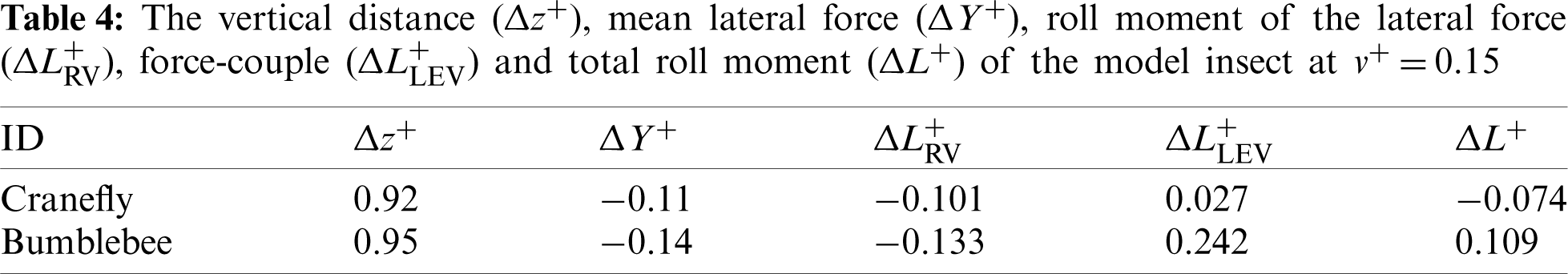
According to the results of analysis above, under the side wind, for the model cranefly, the CLV-effect is weaker than the CRV-effect, meaning the positive contribution given by the CLV-effect is small; thus, the net roll moment is negative, and hence the negative derivative Lv+.

3.3 Stability Properties

In this section, the lateral stability properties of the hovering model cranefly are investigated here with the stability derivatives and morphological data given above. Based on the averaging theorem, the dynamic stability could be examined via the eigenvalues and eigenvectors of its matrix A. For the model cranefly, the results of eigenvalues and eigenvectors showed in Tab. 5 indicate three lateral motion modes.

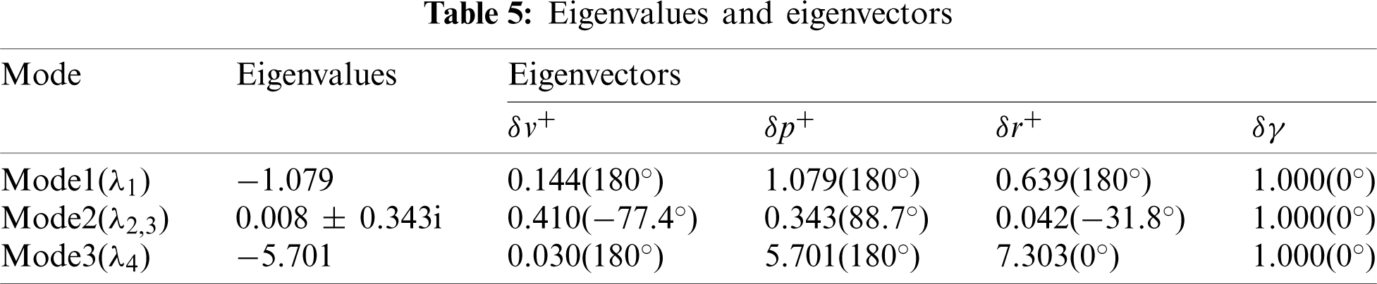
Mode 1 corresponds to a stable subsidence mode with a negative real eigenvalue (λ1). In this natural mode, the motion is a combination of δv+, δp+ and δr+, and the magnitudes of δv+ and δr+ is much smaller than that of δp+, while the phase angle of three of them are the same. Mode 2 has a pair of complex conjugate eigenvalues with positive real part (λ2,3), indicating an unstable oscillatory mode, in which the dominate state variables are δv+ and δp+, and the motion of v+ is in antiphase with that of p+. Noted that the positive real part is very small, the instability of the unstable oscillatory mode is quite weak, which could be seen from the characteristic time constant of Mode 2. Here, for the weakly unstable mode, the time for the initial disturbance to double tdouble (tdouble=0.693/n^, n^ is the real part of the complex eigenvalue) is up to tens of times of wingbeat period, meaning it would take a relatively long time to double the amplitude. Mode 3 also corresponds to a negative real eigenvalue (λ4), but a large magnitude compared to that of eigenvalue λ1, resulting in that the stable subsidence mode would converge faster with an extraordinary small time constant to reach half the value of initial disturbance. In this natural mode of motion, the main state variables are δp+ and δr+, which are out of phase.

It can be seen from the above analysis that, comparing with the hovering bumblebee model [11], the modal structure of cranefly is different. Due to the weakly unstable mode, the lateral dynamics of hovering cranefly model is close to neutrally stable. Xu et al. [16] reported that the weakly unstable mode is chiefly due to the derivative Lv+. Here, the sign of the derivative Lv+ is inverted from positive to negative (for bumblebee [11], the sign of Lv+ is positive); additionally, if the derivative Lv+ is changed to be a larger positive value, and the other derivatives in the system matrix remained unchanged, the recalculated eigenvalues would be similar with those of bumblebee [11].

3.4 Discussion on the Stability Characterization

In the literatures, different aerodynamic models with different fidelity levels, the quasi-steady model [7,9,12,17] and the CFD method [8,11,13,16], are commonly applied to acquire the stability derivatives and identify the dynamic stability for various hovering insects in the lateral direction. This section focuses on comparisons of the lateral stability characteristics in this paper and some previous studies.

For the quasi-steady aerodynamic models, the lateral motion of hovering insects is stable due to the negative roll moment derivative [7,9,12,17]. Herein the sign of the roll moment derivative for hovering cranefly is also negative, and the dynamic modal structure includes one weakly unstable oscillatory mode. In other words, the lateral motion of hovering cranefly can be considered as nearly neutral. The recent study [17] has pointed that the wing-wing interaction has the effect on the roll moment derivative, which can turn to be negative compared with the case without the wing-wing interaction and stabilize the hovering hawkmoth in lateral. Considering that the flows around the right and left wing herein are calculated separately, therefore, the value of the negative roll moment derivative Lv+ of hovering cranefly may become larger if the wing-wing interaction is taken into account. When changing the derivative Lv+ from −0.967 to −1.230 artificially (the absolute value is equal to that of the roll moment derivative of bumblebee, shown in Tab. 3), the recalculated eigenvalues are −1.099, 0.023 ± 0.384i and −5.739. Therefore the dynamic modal structure of hovering cranefly remains the same.

For the previous CFD studies, the dynamic modal structure of cranefly, including one weakly unstable oscillatory mode and two subsidence modes, is different from those of hovering dronefly [8], bumblebee [11] and mosquito [13], while similar to that of hovering honeybee [16]. The reason for the difference has been briefly discussed in the above section, which is the derivative Lv+ with different sign (for dronefly [8], bumblebee [11] and mosquito [13], the signs of Lv+ are positive) causing the modal structure to change. However, the signs of derivative Lv+ of hovering honeybee and cranefly are both negative, thus the same modal structures are possessed. When insects moving laterally, the CLV-effect and the CRV-effect make positive and negative contributions on the derivative Lv+, respectively, the relative strength of which determined the sign of the derivative. For hovering dronefly, bumblebee and mosquito, the CLV-effect is stronger than the CRV-effect, meaning the positive roll moment is bigger than the negative roll moment, and hence the positive derivative Lv+ [8,11,13]. For hovering honeybee, it is the relatively large vertical distance (Δz+) that enhanced the CRV-effect, which makes the negative contribution bigger on the derivative Lv+ [16]. For hovering cranefly, the previous comparative analysis in Section 3.2 has pointed that the CLV-effect is weaker, meaning the positive contribution is smaller. Thus, the net roll moment is negative, and hence the negative derivative Lv+. Note that the aspect ratio of cranefly (AR = 5.5) is relatively large and the Reynolds number (Re = 240) is relatively small, and the different morphological parameter and Reynolds number could have an impact on the aerodynamic characteristics, and further influence the CLV-effect. Although the aspect ratio of the mosquitoes is also relatively large (AR = 5), they use different aerodynamic mechanisms due to the rather short stroke amplitude [14] while much more insects use the same delayed-stall mechanism. Thus, for insects using the delayed-stall mechanism, when the lateral winds acting on the flapping wings, the influence on the CLV-effect made by the different morphological and kinematic parameters (Reynolds number) still unclear and need further investigation.

4  Conclusions

(1) This paper investigated the lateral dynamics of a model cranefly in hover. The lateral disturbance motion of model cranefly in hover consists of three natural modes, and the flight in lateral is nearly neutral, that is different from most other insects.

(2) The neutral stability is chiefly due to the stability derivative Lv+, the sign of which is negative, quite different from most other insects. When model cranefly moving laterally, the relative strength of the two flow effects acting on the flapping wings simultaneously is different from that of bumblebee, and the CLV-effect is weaker than the CRV-effect, meaning the magnitude of positive roll moment contributed by the CLV-effect is much smaller than the negative counterpart contributed by the CRV-effect, thus the sign of derivative Lv+ is inverted from normal positive to negative.

(3) The stability analysis on model cranefly shows that, during normal-hovering flight, the stability property of lateral disturbance motions is not as robust as that of longitudinal motion, and owing to the opposite sign of Lv+, insects with different morphological and kinematic parameters in the natural world may possess different modal structure and stability characteristics.

Funding Statement: This work was supported by grants from the National Natural Science Foundation of China (Nos. 11802262 and 11502228).

Conflicts of Interest: The authors declare that they have no conflicts of interest to report regarding the present study.

This work is licensed under a Creative Commons Attribution 4.0 International License, which permits unrestricted use, distribution, and reproduction in any medium, provided the original work is properly cited.