| Computer Modeling in Engineering & Sciences |
DOI: 10.32604/cmes.2021.016159
ARTICLE
Numerical Implementation of a Unified Viscoplastic Model for Considering Solder Joint Response under Board-Level Temperature Cycling
Department of Mechanical Engineering, National Cheng Kung University, Tainan, 701, Taiwan
*Corresponding Author: Tz-Cheng Chiu. Email: tcchiu@mail.ncku.edu.tw
Received: 12 February 2021; Accepted: 29 April 2021
Abstract: An implicit integration scheme was developed for simulating the viscoplastic constitutive behavior of Sn3.0Ag0.5Cu solder and programmed into a user material subroutine of the finite element software ANSYS. The numerical procedure first solves the essential state variables by using a three-level iterative procedure, and updates the remaining stress and state variables accordingly. The numerical implementation was applied to consider the responses of solder joints in an electronic assembly under temperature cycling condition. The viscoplastic strain energy density accumulation over one temperature cycle was identified as a feasible parameter for evaluating the thermomechanical reliability of the solder joints.
Keywords: Pb-free; hysteresis; ratcheting; fatigue; tangent modulus
In state-of-the-art microelectronic assemblies, the individual integrated-circuit (IC) components are connected to the printed-circuit board (PCB) through arrays of solder joints. Under service conditions involving repetitive temperature changes, the mismatch between the coefficients of thermal expansion (CTEs) of the PCB and IC components leads to thermomechanical fatigue and failure of the electronic assembly. The solder joint, which is the electrical as well as the structural interconnection between the component and PCB, is typically the weakest link from the perspective of thermomechanical reliability. Accurate prediction of the solder joint response is therefore imperative to the reliability modeling of the electronic assembly. In order to achieve that, the simulation should be able to consider the constitutive behavior of the solder under service conditions. One of the standard solder materials used in the board-level assembly is the Pb-free Sn3.0Ag0.5Cu (96.5 wt.% Sn, 3.0 wt.% Ag, 0.5 wt.% Cu) alloy which has a melting temperature of 217
The mathematical form of the unified viscoplastic model is typically a set of nonlinear first-order differential equations, and the corresponding thermomechanical problem is solved by using nonlinear finite element (FE) procedure. In the FE procedure for analyzing the viscoplastic problem, the stress equilibrium is expressed in the form of nonlinear virtual work equations. The process of obtaining the nodal displacements involves applying the load in a sequence of discrete time steps and solving the global nonlinear equilibrium equations at each incremental step by Newton-Raphson iteration. During each global equilibrium iteration, values of new stresses and internal state variables at each Gaussian integration points are calculated for the prescribed strain increment and temperature change. These results are then used to determine the residual force vector and the material tangent stiffness for the FE stiffness matrix. The calculations of the new stresses and state variables at Gaussian integration points are performed with a time-integration scheme of the viscoplastic model. In the integration scheme, the coupled and nonlinear differential constitutive equations are discretized in a strain-driven format. Time-integration procedures based on non-iterative forward-Euler scheme had been adopted for the viscoplastic model due to their easy implementation [10,11]. A disadvantage of the explicit scheme is that the time increment is severely restricted because of numerical stability requirements. To overcome this issue, semi-implicit time-integration schemes were developed to improve stability and to retain numerical simplicity. These semi-implicit procedures [12–14] calculate the forward gradient of the relevant constitutive function by using Taylor series expansion at the initial state. These semi-implicit approaches are non-iterative and provide improvements over the explicit procedures. However, it is still important to control the time increment carefully because the accuracy of the forward gradient method may be severely affected by the time step size, especially in rapid-changing deformation regimes [14]. Fu et al. [15] developed another semi-implicit time-integration approach. In this procedure, the effective viscoplastic strain increment is evaluated by using real implicit integration method while the other state variables are obtained by explicit update. Similar approach was adopted to address the integration problem for a damage-coupled unified viscoplastic model [16].
Fully-implicit backward Euler schemes had also been implemented in time-integration procedures for viscoplastic models [17–27]. Because of the unconditional stability in time step size, it is possible to improve the computational efficiency of these schemes without much loss in solution accuracy. In the implicit scheme, nonlinear equations of the new stress and other state variables are derived from the constitutive equations, and then transformed to a set of nonlinear algebraic equations of the unknown variables. Iterative procedures were usually applied to solve the system of nonlinear equations. Because the iterative solutions are performed at every Gaussian integration point for each time step, the computation cost would be very significant if the number of unknowns is higher than the essentially independent variables in the constitutive model, especially when tensor-valued internal state variables are used [17,18]. For improving the computation efficiency, efforts had been focused on simplifying the discretized nonlinear system of equations such that the number of unknowns is reduced to the same as the number of independent variables in the corresponding constitutive model [19–25,27]. Hartmann et al. [19,20] showed that, for plastic and viscoplastic models with multiple Armstrong-Frederick kinematic hardening terms, the nonlinear system of equations can be reduced to one scalar nonlinear equation for calculating the new state variables. By following a similar derivation, Kobayashi et al. [21] demonstrated that the implicit integration of kinematic-hardening plastic model consisting strain hardening and dynamic recovery terms can also be reduced to solving a scalar nonlinear equation. The approach was also applied to reduce the number of equations for more complicated constitutive models [22–24].
Aside from the discretized form of the constitutive equations, the robustness of the numerical solution is also influenced by the iterative procedure. In general, Newton-Raphson iteration can readily be adopted for solving the equations. However, for handling equations of high nonlinearity, designs of appropriate local iterative schemes were proposed [18,21,22,24–26]. Saleeb et al. [18] applied line-search strategy to improve the robustness of the Newton-Raphson iterative solution. Kobayashi and coworkers adopted a successive substitution method for solving nonlinear scalar constitutive equations [21,22]. Multi-level iteration strategies were also adopted for solving the discretized nonlinear constitutive equations: Kullig et al. [24] presented a two-level iteration strategy by combing Pegasus method and fixed-point iteration to solve a system of three coupled nonlinear equations, Lush et al. [25] developed a two-level iteration strategy that combines the Newton-Raphson procedure with bracketing method for obtaining good global convergence.
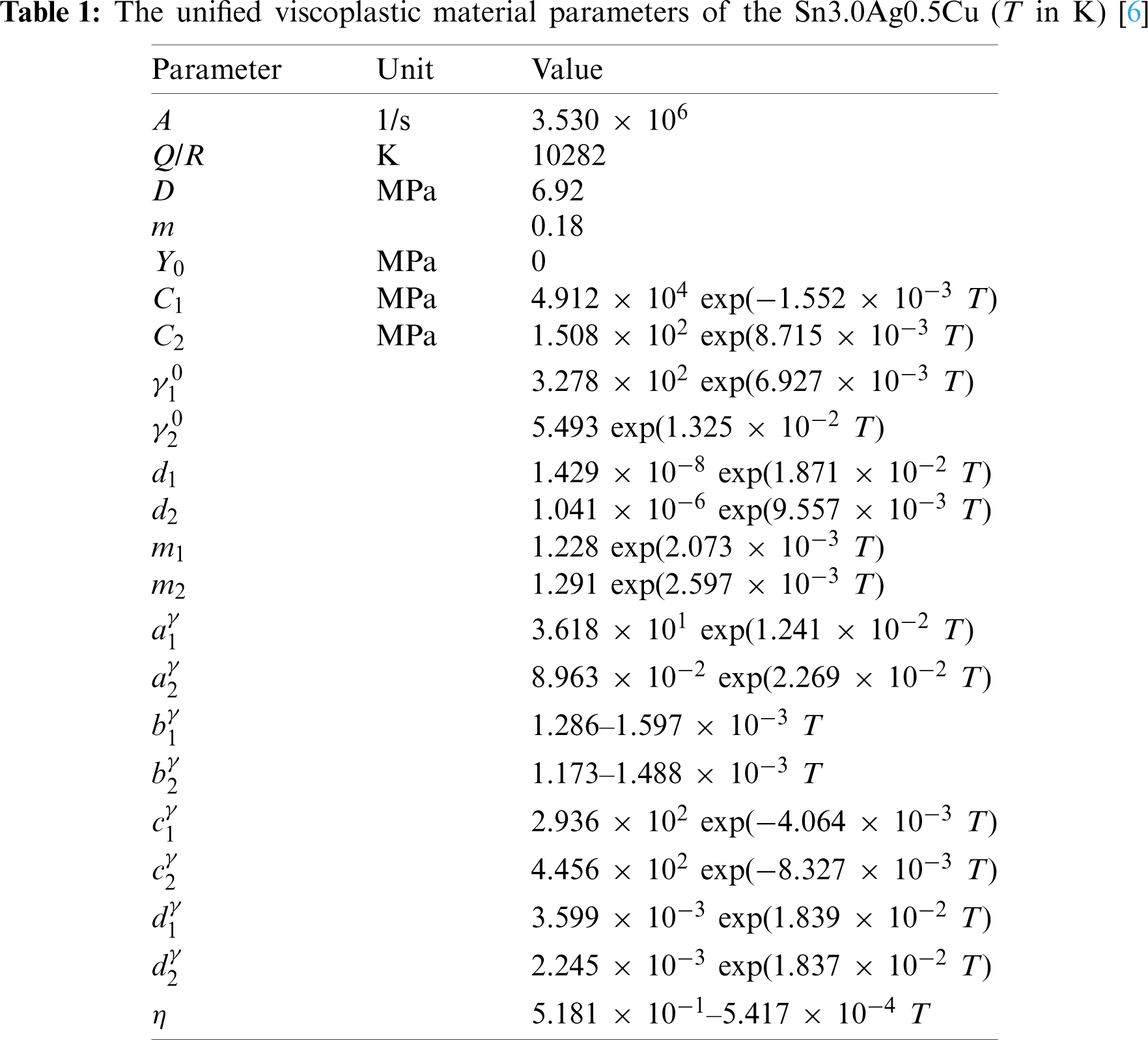
In this paper, a fully-implicit time-integration scheme is presented for a novel viscoplastic constitutive model of Sn3.0Ag0.5Cu solder [6]. The viscoplastic model, which was proposed by the authors of this paper, was first discretized and reduced to a set of four coupled nonlinear zero-form equations for the four essentially independent variables. A multi-level iteration strategy was implemented for solving this set of nonlinear equations. The implicit integration scheme was programmed for the user-defined material subroutine USERMAT in commercial FE software ANSYS [28] to perform local computation. For each current load step in the global equilibrium iteration, new local stress and state variables at every Gaussian integration point are calculated from the given strain and temperature increments. Furthermore, the consistent tangent stiffness was also derived and programmed into the USERMAT. It is used for preserving the quadratic convergence of the global Newton–Raphson equilibrium iteration [29,30]. The FE simulations of solder bar under strain- or stress-controlled uniaxial cyclic loadings were conducted in ANSYS with the USERMAT subroutine, and compared to experimental results for validating the implementation. The USERMAT subroutine is also applied to consider the thermomechanical responses of the ball grid array (BGA) Sn3.0Ag0.5Cu solder joints in an electronic assembly under temperature-cycling reliability test condition.
From experimental characterizations under monotonic and cyclic loading conditions, a kinematic hardening rule based viscoplastic model was developed for the Sn3.0Ag0.5Cu alloy [6]. The main features incorporated in the model include dynamic recovery function for considering cyclic softening and static recovery term for considering relaxation under monotonic loading. A brief description of the constitutive model is given in this section.
Within the framework of unified viscoplasticity, the strain tensor can be expressed as
where
where
where
where
where
The flow equation of the unified viscoplastic model is given by
where
In Eq. (7), A, D, m, Q/R and Y0 are material parameters,
The internal state variable of the viscoplastic model is the back stress,
where
where Ci, di, and mi are the material parameters,
where
where
where
The unified viscoplastic model described in Eqs. (6)–(15) consists 22 material parameters: A, Q/R, D, m, Y0,
The unified viscoplastic model described in Section 2 is discretized for numerical FE implementation by using an implicit backward-Euler integration scheme. Details of the time discretization, the numerical integration procedure, the approach for solving the nonlinear algebraic equations and the formulation of the consistent tangent modulus are given as follows.
3.1 Backward Euler Integration Scheme
In the FE procedure, the viscoplastic model, given as a system of nonlinear first-order differential equations, is integrated for a prescribed strain increment to update the stresses and state variables at the Gaussian integration points by using the implicit backward-Euler integration scheme. In this scheme, the time discretization of a general first-order differential equation
where the subscripts n and
Given that the stresses and state variables are known at time tn, the stress increment for a prescribed strain increment can be calculated from the discretized form of Eq. (4), given by
It is emphasized in Eq. (17) that
where
Eq. (18) leads to a predictor-corrector approach which is also known as the return mapping method [32,33]. In this approach, the stress is first estimated by the trial stress, which is calculated by substituting the prescribed
where
The discretization of the viscoplastic model in the backward-Euler form is given as follows. The discretized flow equations corresponding to Eqs. (6)–(8) are given by
The discretized back stress equation corresponding to Eq. (10) is given by
The evolution equation of the dynamic recovery parameter corresponding to Eq. (11) is given by
The strain-memory-surface related evolution equations corresponding to Eqs. (13) and (14) are given by
The discretization of the constitutive equations leads to a set of 26 unknowns:
The effective stress at the new state can be obtained from Eqs. (21) and (24), and is given by
where
Eq. (29) can be converted to a scalar equation by calculating the von-Mises invariant of the effective stress tensor [20,24], which is given by
where
An additional equation for
It can be seen from Eq. (35) that q equals to
By substituting Eq. (36) into Eq. (35) and through some algebraic manipulations, it can be shown that
where
A nonlinear algebraic system consisted of four essential zero-form scalar equations for
The evaluations of the 26 unknowns
3.2 The Time-Integration Procedure
The flow chart of the time-integration procedure is shown in Fig. 1. The time-integration procedure is used for calculating the stresses, strains, viscoplastic strains and other state variables at time tn+1 from the known values at time tn and the incremental time, strain and temperature steps. In this procedure, the trial stresses
The second step in the time-integration procedure is to update the back stresses for the assumed purely elastic state. Under the assumed elastic state, the viscoplastic strain norm increment,
The zero-form equations that are used for solving

Figure 1: The time-integration procedure
The solutions of Eqs. (43) and (44) can be obtained by using the Newton-Raphson method. In this iterative procedure, initial guesses of
where the superscript “int” denotes the initial guess. Once
where
3.3 Solution of the Nonlinear Algebraic System
Among the 4 unknowns to be solved from the simultaneous Eqs. (38)–(41), the orders of

Figure 2: The multi-level iteration scheme
In Eqs. (47) and (48),
For each Level-1 iteration of evaluating f1 and updating
Eq. (49) is expected to have a value greater than zero when
Once the Level-3 iterative solution for
For the iterative solution at each level iteration, it is considered as converged if the following condition is met:
where y represents the variable to be solved, the subscript k denotes the number of the current iteration.
3.4 Consistent Tangent Modulus
The consistent tangent moduli are typically used in nonlinear FE procedures to preserve the rate of convergence in the Newton-Raphson solution for the global equilibrium equations in nonlinear problems. However, it does not affect the accuracy of the global iterative solution [30]. The consistent tangent modulus is obtained by linearizing the stress expression with respect to the mechanical strain increment. In this study, derivation of the consistent tangent modulus is conducted by following the procedures proposed by Kobayashi et al. [22] and Akamatsu et al. [27]. In the derivation, the differentials of the viscoplastic strain increment and the back stress are first expressed, respectively, as
where
where g is a function of the von-Mises invariant of the effective stress and temperature. Because the temperature is prescribed as the input in the time-integration procedure, the differential of
where the differential
The differential
From Eqs. (51) and (56), it can be shown that
where
For determining
where
In Eq. (60),
The differential
By comparing Eqs. (52) and (59), it can be shown that
where
The
By substituting Eq. (52) into Eq. (51) and rearranging, it gives
From Eqs. (18) and (19), the differential stress can be expressed as
where
The deviatoric part of the differential stress can be expressed as
where
By substituting Eq. (72) into Eq. (69), the differential viscoplastic strain increment can be expressed as
By further substituting Eq. (74) into Eq. (70), the consistent tangent modulus can be written as
The time-integration scheme and the consistent tangent modulus of the viscoplastic constitutive model was implemented as a USERMAT subroutine in the FEM software ANSYS. Numerical results of the Sn3.0Ag0.5Cu solder rod under cyclic loadings were first obtained and validated to the experimental data. The numerical model is then applied to simulate the responses of BGA solder joints under temperature cycling condition.
4.1 Solder Rod under Mechanical Cycling
The responses of Sn3.0Ag0.5Cu solder rod under uniaxial cyclic loadings at constant temperatures of 25, 75 or 125

Figure 3: Finite element model of the solder rod under uniaxial cyclic loading
The FE model was first applied to consider the solder response under cyclic straining with a constant rate of 2
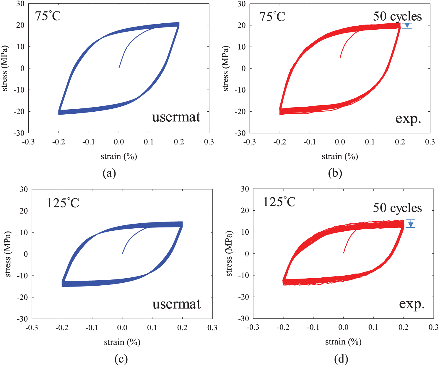
Figure 4: Solder responses under cyclic straining with strain range of
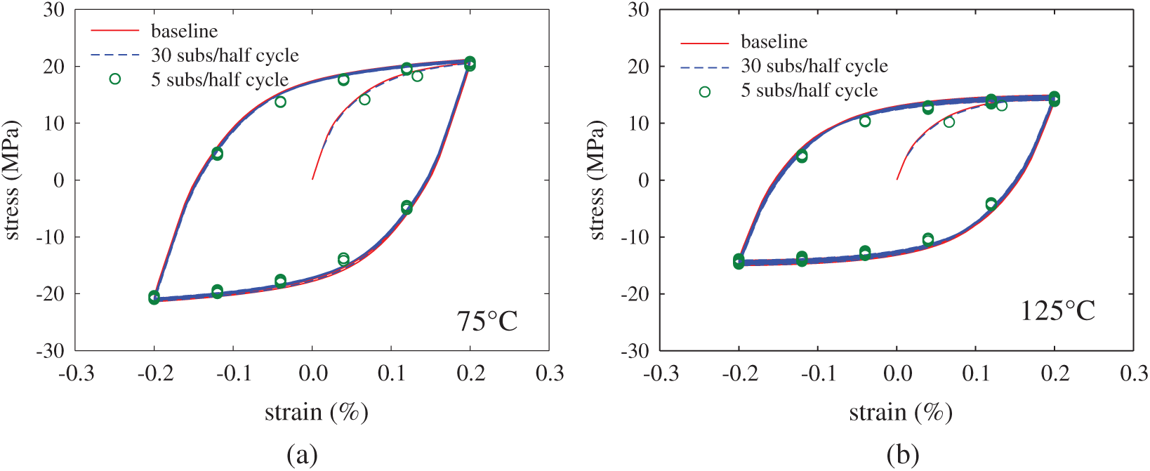
Figure 5: Effect of solution step size on simulation results for cyclic straining under strain range of
The cyclic response of the solder rod under a triangular strain wave of range 0%–0.25% was also considered by using the FE model shown in Fig. 6. The cyclic loading was applied at a constant strain rate of 2
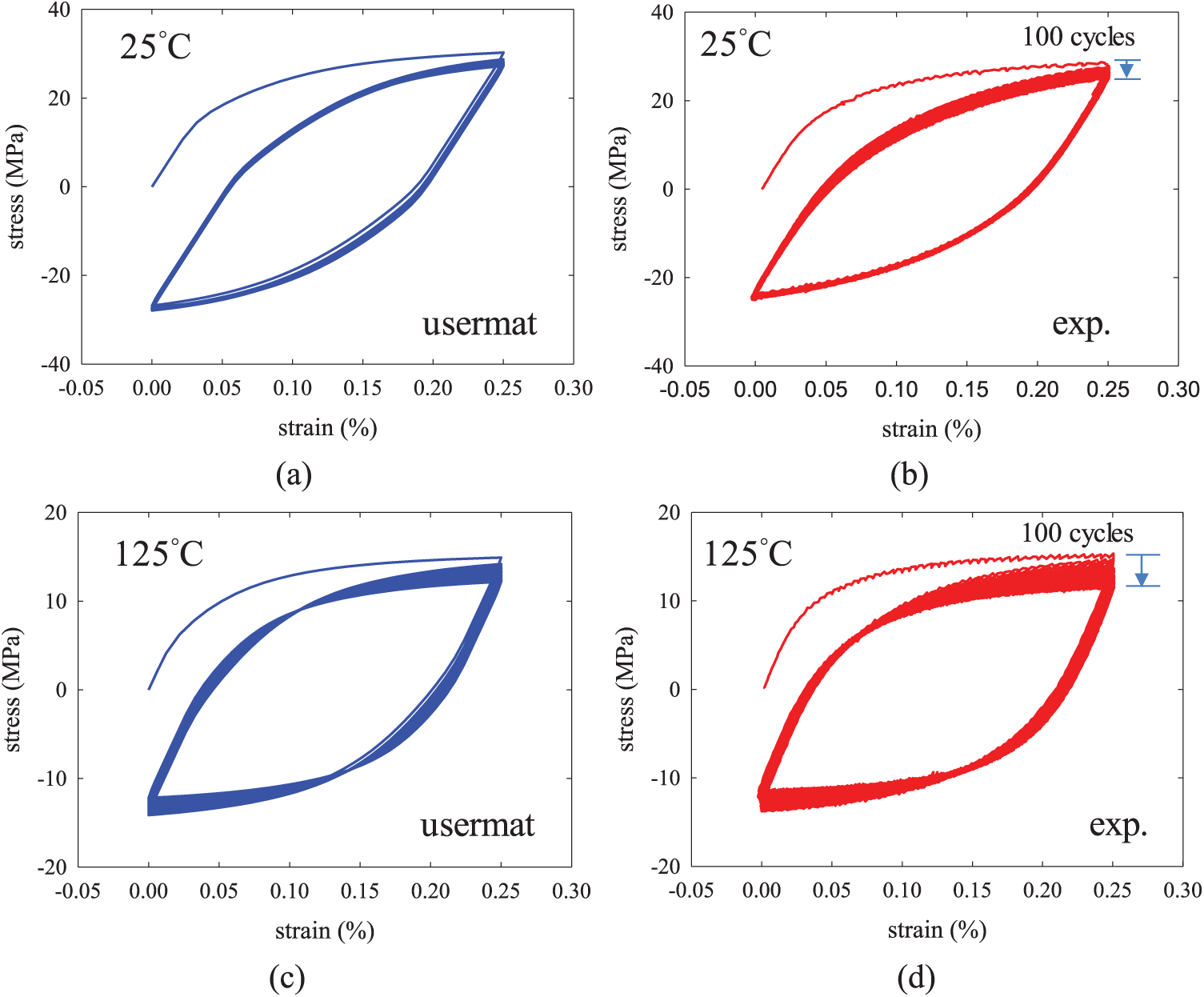
Figure 6: Solder responses under cyclic straining with strain range of 0%–0.25%, (a) simulation result, at 25
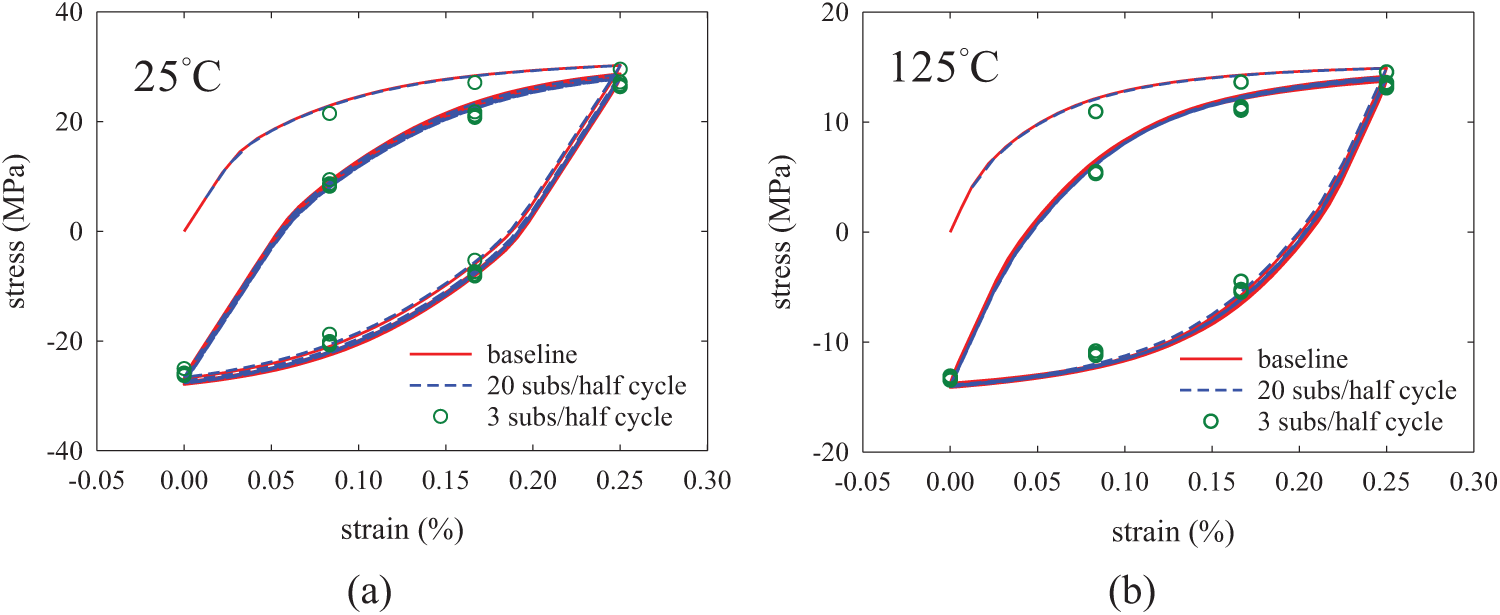
Figure 7: Effect of solution step size on simulation results for cyclic straining under strain range of 0%–0.25%, (a) at 25
The ratcheting response of the Sn3.0Ag0.5Cu rod under cyclic stress loading at constant temperature of 75
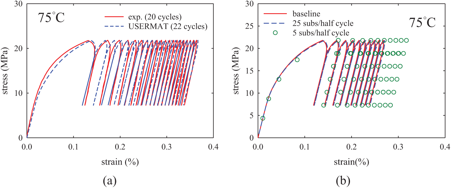
Figure 8: Ratcheting responses under cyclic stressing test at 75
In the cases of uniform steps, the sub-step numbers of 5 and 25 were considered. Shown in Fig. 8 are the results of the ratcheting simulations. The comparison of the automatic time-stepping solution to the experimental results is shown in Fig. 8a, from which it can be seen that the numerical results correlate well to the experimental data. The effect of time-stepping strategy on the numerical ratcheting solution is shown in Fig. 8b. It can be seen from Fig. 8b that the 25-sub-step procedure gives stress solutions practically the same as the automatic time-stepping solution, which is denoted as the baseline. On the other hand, the 5-sub-step procedure clearly over-estimates the ratcheting strain, especially for the first few cycles. The poor numerical result for the 5-sub-step case can be attributed to the low tangent modulus of the solder, which would lead to a higher simulation error when large stress step is assigned in the incremental strain-based iterative scheme. A similar observation was also made in [23]. From the comparisons of the numerical results shown in Figs. 5, 7 and 8, it can be seen that the incremental step size has a stronger influence on the numerical solutions of the stress-controlled problems than that of the strain-controlled problems.
4.2 BGA Solder Joints under Temperature Cycling
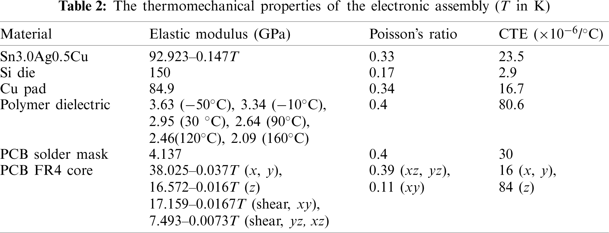
The viscoplastic responses of the BGA Sn3.0Ag0.5Cu solder joints in the assembly of a wafer-level package (WLP) on PCB under a standard −40
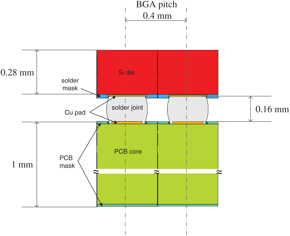
Figure 9: The cross-section schematic of a WLP assembled on PCB
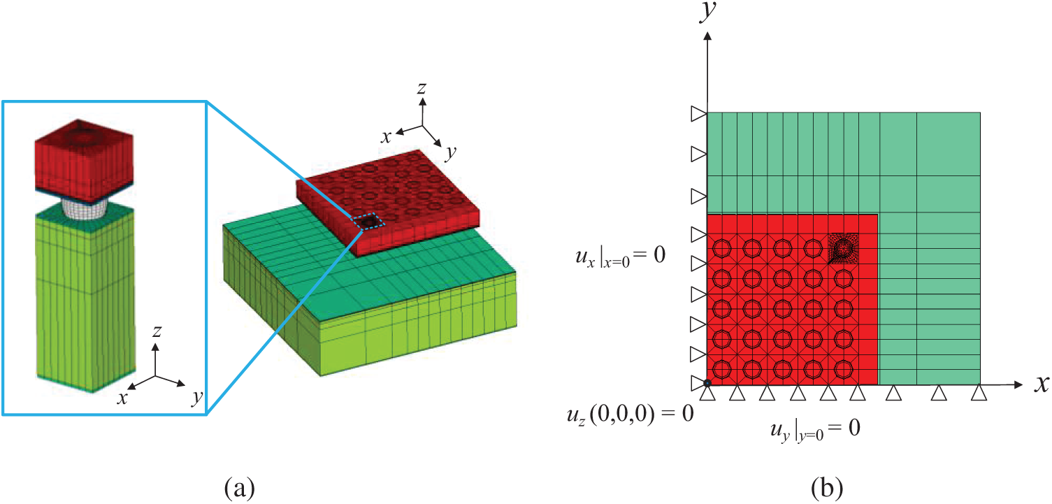
Figure 10: Finite element model of the WLP assembled on PCB (a) the submodeling FE mesh, (b) boundary conditions
Shown in Fig. 13 is the −40
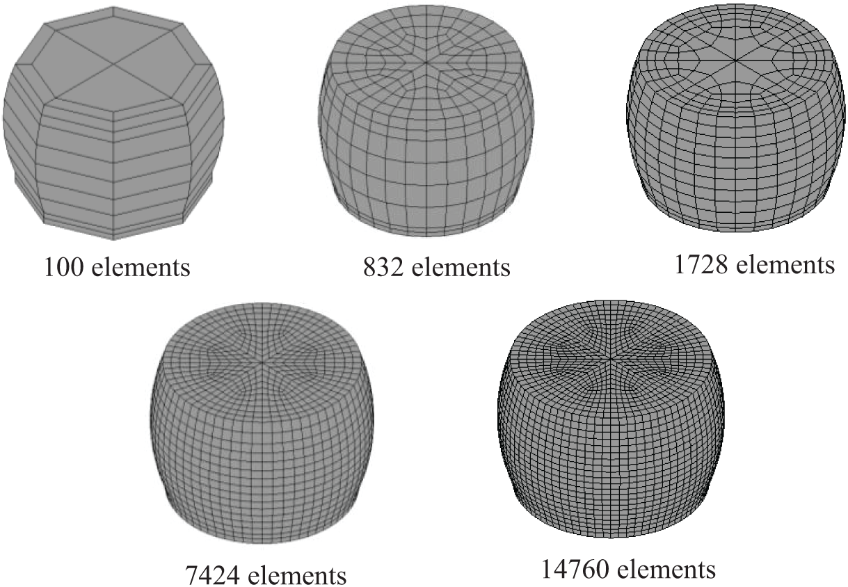
Figure 11: Various meshes of the critical solder joint

Figure 12: The von-Mises stress contour of the critical solder joint
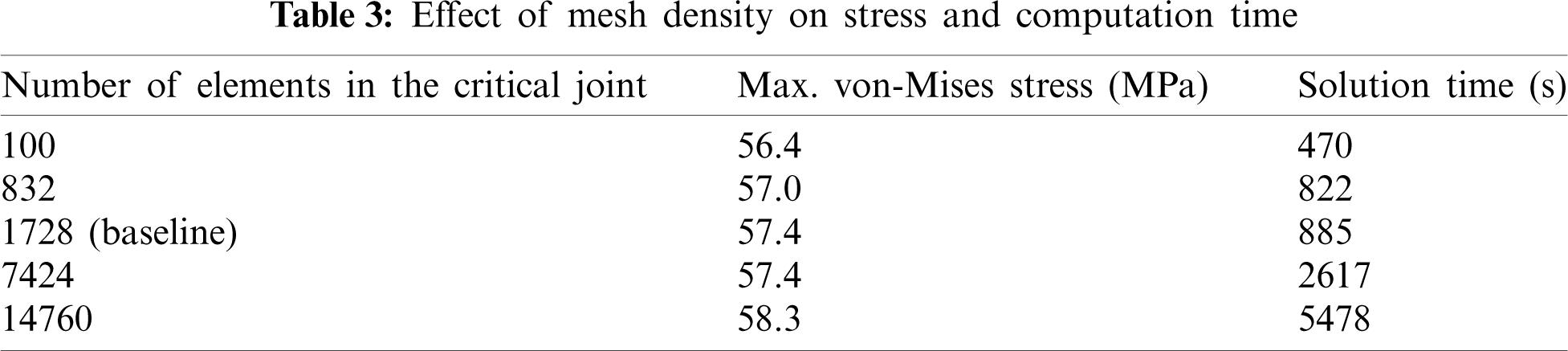
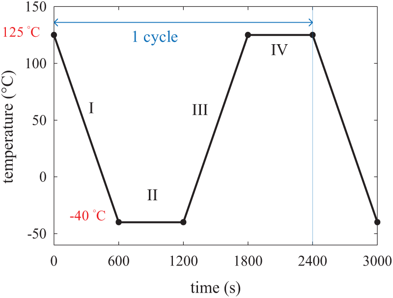
Figure 13: The −40
The von-Mises stress distribution in the critical solder joint at the end of the cooling stage of the 11th cycle is shown in Fig. 14. Because the thermal strain is the highest at −40
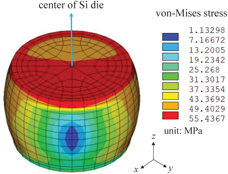
Figure 14: von-Mises stress distribution in the critical solder joint
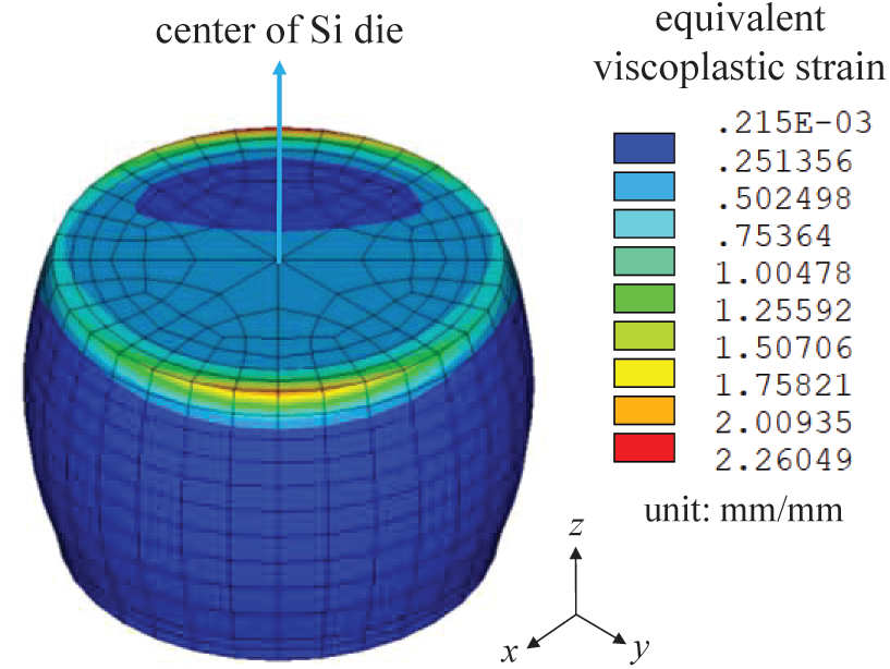
Figure 15: Equivalent viscoplastic strain in the critical solder joint
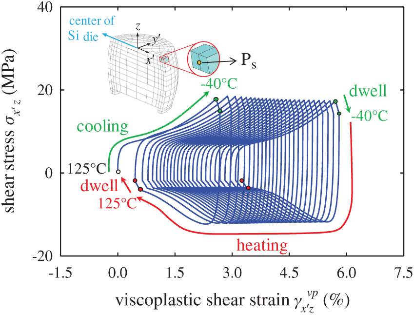
Figure 16: Shear stress-viscoplastic shear strain relationship at the point Ps
In addition to the stress and strain solutions, the viscoplastic strain energy density is another parameter considered extensively in the semi-empirical approaches for predicting temperature cycling reliability of solder joints [36,37]. The viscoplastic strain energy density is given by
The viscoplastic strain energy density is evaluated at each element in an incremental fashion. For each solution sub-step, the viscoplastic strain energy density increment is calculated in the USERMAT subroutine by using trapezoidal integration. The volume-averaged viscoplastic strain energy density is defined as
where V is the volume of the element. By following Darveaux’s approach [37], the volume-averaged viscoplastic strain energy density (
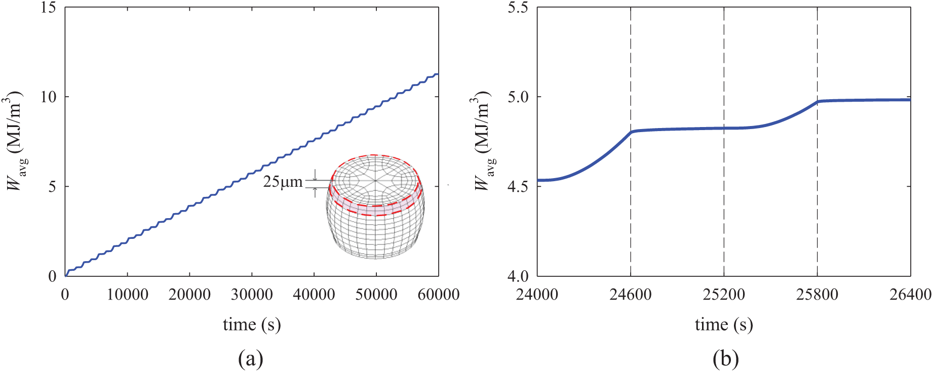
Figure 17: The volume-averaged viscoplastic strain energy density near the package-solder interface (a) the evolution over time, (b) zoom-in at the 11th cycle
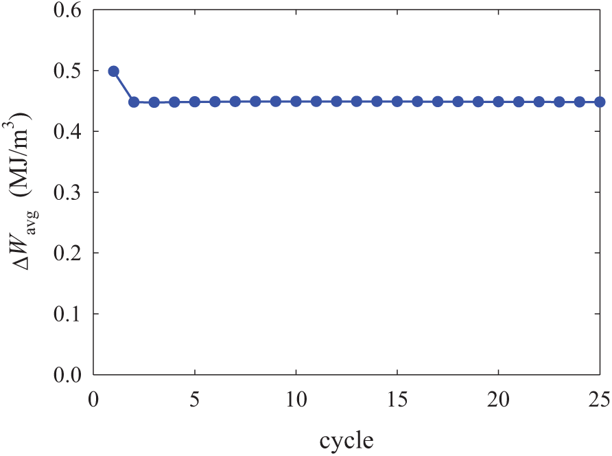
Figure 18: The volume-averaged viscoplastic strain energy density increment per cycle
A fully implicit integration procedure was developed for a unified viscoplastic constitutive model and implemented as a user-defined material subroutine (USERMAT) in the commercial FE software ANSYS. In the numerical implementation, a Chaboche framework based viscoplastic model that considers the cyclic softening behavior of Sn3.0Ag0.5Cu solder was first discretized as a set of nonlinear system of equations for 26 unknowns. Additional simplification was applied to reduce the nonlinear system to solving four equations for four essential variables. The implicit integration scheme first solves the four essential variables by using a three-level, Newton-Raphson and Pegasus method based iterative procedure, and updates the remaining stresses and state variables accordingly. A consistent tangent modulus for the constitutive equation was also derived and implemented in the USERMAT subroutine. Validation of the USERMAT was accomplished by simulating the solder rod responses under either strain-or stress-controlled cycling and compared to experimental measurements. It was shown that the numerical model is capable of predicting the softening response under cyclic straining and the ratcheting response under cyclic stressing. A FE model of WLP connected to PCB through BGA solder joints was also developed to simulate the solder joint response under board-level temperature cyclic condition. From the simulation, the viscoplastic strain energy density accumulation over one temperature cycle was identified as a feasible parameter for evaluating the thermomechanical reliability of the of solder joints in electronic assembly.
Funding Statement: This study was supported by the Ministry of Science and Technology, ROC, under the Grants MOST 107-2221-E-006-138 and MOST 109-2221-E-006-008 MY2.
Conflicts of Interest: The authors declare that they have no conflicts of interest to report regarding the present study.
1. Stouffer, D. C., Dame, L. T. (1996). Inelastic deformation of metals: Models, mechanical properties, and metallurgy. New Jersey, USA: John Wiley & Sons. [Google Scholar]
2. Chaboche, J. L. (2008). A review of some plasticity and viscoplasticity constitutive theories. International Journal of Plasticity, 24(10), 1642–1693. DOI 10.1016/j.ijplas.2008.03.009. [Google Scholar] [CrossRef]
3. Wippler, S., Kuna, M. (2008). Experimental and numerical investigation on the reliability of leadfree solders. Engineering Fracture Mechanics, 75(11), 3534–3544. DOI 10.1016/j.engfracmech.2007.03.046. [Google Scholar] [CrossRef]
4. Kuna, M., Wippler, S. (2010). A cyclic viscoplastic and creep damage model for lead free solder alloys. Engineering Fracture Mechanics, 77(18), 3635–3647. DOI 10.1016/j.engfracmech.2010.03.015. [Google Scholar] [CrossRef]
5. Metais, B., Kabakchiev, A., Maniar, Y., Guyenot, M., Metasch, R. et al. (2015). A viscoplastic-fatigue-creep damage model for tin-based solder alloy. Proceedings of the 16th International Conference on Thermal, Mechanical and Multi-Physics Simulation and Experiments in Microelectronics and Microsystems. Budapest. [Google Scholar]
6. Yang, H. C., Chiu, T. C. (2021). A unified viscoplastic model for characterizing the softening behavior of the Sn3.0Ag0.5Cu solder under monotonic and cyclic loading conditions. Microelectronics Reliability, 119(5), 114086. DOI 10.1016/j.microrel.2021.114086. [Google Scholar] [CrossRef]
7. Long, X., He, X., Yao, Y. (2017). An improved unified creep-plasticity model for SnAgCu solder under a wide range of strain rates. Journal of Materials Science, 52(10), 6120–6137. DOI 10.1007/s10853-017-0851-x. [Google Scholar] [CrossRef]
8. Wang, W. J., Long, X., Du, C. Y., Fu, Y. H., Yao, Y. et al. (2019). Enhancement of the unified constitutive model for viscoplastic solders in wide strain rate and temperature ranges. Strength of Materials, 51(6), 917–925. DOI 10.1007/s11223-020-00142-5. [Google Scholar] [CrossRef]
9. Long, X., Chen, Z. B., Wang, W. J., Fu, Y. H., Wu, Y. P. (2020). Parameterized Anand constitutive model under a wide range of temperature and strain rate: Experimental and theoretical studies. Journal of Materials Science, 55(24), 10811–10823. DOI 10.1007/s10853-020-04689-1. [Google Scholar] [CrossRef]
10. Zienkiewicz, O. C., Cormeau, I. C. (1974). Visco-plasticity-plasticity and creep in elastic solids–A unified numerical solution approach. International Journal for Numerical Methods in Engineering, 8(4), 821–845. DOI 10.1002/nme.1620080411. [Google Scholar] [CrossRef]
11. Kumar, V., Morjaria, M., Mukherjee, S. (1980). Numerical integration of some stiff constitutive models of inelastic deformation. Journal of Engineering Materials and Technology, 102(1), 92–96. DOI 10.1115/1.3224791. [Google Scholar] [CrossRef]
12. Peirce, D., Shih, C. F., Needleman, A. (1984). A tangent modulus method for rate dependent solids. Computers & Structures, 18(5), 875–887. DOI 10.1016/0045-7949(84)90033-6. [Google Scholar] [CrossRef]
13. Tanaka, T. G., Miller, A. K. (1988). Development of a method for integrating time-dependent constitutive equations with large, small or negative strain rate sensitivity. International Journal for Numerical Methods in Engineering, 26(11), 2457–2485. DOI 10.1002/nme.1620261107. [Google Scholar] [CrossRef]
14. Busso, E. P., Kitano, M., Kumazawa, T. (1994). A forward gradient time integration procedure for an internal variable constitutive model of Sn-Pb solder. International Journal for Numerical Methods in Engineering, 37(4), 539–558. DOI 10.1002/nme.1620370402. [Google Scholar] [CrossRef]
15. Fu, C., McDowell, D. L., Ume, I. C. (1998). A finite element procedure of a cyclic thermoviscoplasticity model for solder and copper interconnects. Journal of Electronic Packaging, 120(1), 24–34. DOI 10.1115/1.2792281. [Google Scholar] [CrossRef]
16. Wei, Y., Chow, C. L., Neilsen, M. K., Fang, H. E. (2003). Failure analysis of solder joints with a damage-coupled viscoplastic model. International Journal for Numerical Methods in Engineering, 56(14), 2199–2211. DOI 10.1002/nme.660. [Google Scholar] [CrossRef]
17. Ronda, J., Oliver, G. J. (1998). Comparison of applicability of various thermo-viscoplastic constitutive models in modelling of welding. Computer Methods in Applied Mechanics and Engineering, 153(3–4), 195–221. DOI 10.1016/S0045-7825(97)00069-8. [Google Scholar] [CrossRef]
18. Saleeb, A. F., Wilt, T. E., Li, W. (2000). Robust integration schemes for generalized viscoplasticity with internal-state variables. Computers & Structures, 74(5), 601–628. DOI 10.1016/S0045-7949(99)00020-6. [Google Scholar] [CrossRef]
19. Hartmann, S., Haupt, P. (1993). Stress computation and consistent tangent operator using non-linear kinematic hardening models. International Journal for Numerical Methods in Engineering, 36(22), 3801–3814. DOI 10.1002/nme.1620362204. [Google Scholar] [CrossRef]
20. Hartmann, S., Luhrs, G., Haupt, P. (1997). An efficient stress algorithm with applications in viscoplasticity and plasticity. International Journal for Numerical Methods in Engineering, 40(6), 991–1013. DOI 10.1002/(SICI)1097-0207(19970330)40:6¡991::AID-NME98¿3.0.CO;2-H. [Google Scholar] [CrossRef]
21. Kobayashi, M., Ohno, N. (2002). Implementation of cyclic plasticity models based on a general form of kinematic hardening. International Journal for Numerical Methods in Engineering, 53(9), 2217–2238. DOI 10.1002/nme.384. [Google Scholar] [CrossRef]
22. Kobayashi, M., Mukai, M., Takahashi, H., Ohno, N., Kawakami, T. et al. (2003). Implicit integration and consistent tangent modulus of a time-dependent non-unified constitutive model. International Journal for Numerical Methods in Engineering, 58(10), 1523–1543. DOI 10.1002/nme.825. [Google Scholar] [CrossRef]
23. Kang, G. (2006). Finite element implementation of visco-plastic constitutive model with strain-range-dependent cyclic hardening. Communications in Numerical Methods in Engineering, 22(2), 137–153. DOI 10.1002/cnm.803. [Google Scholar] [CrossRef]
24. Kullig, E., Wippler, S. (2006). Numerical integration and FEM-implementation of a viscoplastic Chaboche-model with static recovery. Computational Mechanics, 38(6), 1–13. DOI 10.1007/s00466-005-0704-3. [Google Scholar] [CrossRef]
25. Lush, A. M., Weber, G., Anand, L. (1989). An implicit time-integration procedure for a set of internal variable constitutive equations for isotropic elasto-viscoplasticity. International Journal of Plasticity, 5(5), 521–549. DOI 10.1016/0749-6419(89)90012-0. [Google Scholar] [CrossRef]
26. Johansson, M., Mahnken, R., Runesson, K. (1999). Efficient integration technique for generalized viscoplasticity coupled to damage. International Journal for Numerical Methods in Engineering, 44(11), 1727–1747. DOI 10.1002/(SICI)1097-0207(19990420)44:11¡1727::AID-NME568¿3.0.CO;2-P. [Google Scholar] [CrossRef]
27. Akamatsu, M., Nakane, K., Ohno, N. (2008). Implicit integration by linearization for high-temperature inelastic constitutive models. Journal of Solid Mechanics and Materials Engineering, 2(7), 967–980. DOI 10.1299/jmmp.2.967. [Google Scholar] [CrossRef]
28. ANSYS 17.2 (2016). Guide to user programmable features: USERMAT. Canonsburg, Pennsylvania: Ansys, Inc. [Google Scholar]
29. Simo, J. C., Taylor, R. L. (1985). Consistent tangent operators for rate-independent elastoplasticity. Computer Methods in Applied Mechanics and Engineering, 48(1), 101–118. DOI 10.1016/0045-7825(85)90070-2. [Google Scholar] [CrossRef]
30. Hughes, T. J. R. (1984). Numerical implementation of constitutive models: rate-independent deviatoric plasticity. Theoretical foundation for large-scale computations for nonlinear material behavior mechanics of elastic and inelastic solid, vol. 6, pp. 29–63. Dordrecht, Netherlands: Springer. [Google Scholar]
31. Chaboche, J. L., Dang Van, K., Cordier, G. (1979). Modelization of the strain memory effect on the cyclic hardening of 316 stainless steel. Proceedings of the 5th International Conference on Structural Mechanics in Reactor Technology, Berlin. [Google Scholar]
32. Krieg, R. D., Krieg, D. B. (1977). Accuracies of numerical solution methods for the elastic-perfectly plastic model. Journal of Pressure Vessel Technology, 99(4), 510–515. DOI 10.1115/1.3454568. [Google Scholar] [CrossRef]
33. Ortiz, M., Simo, J. C. (1986). An analysis of a new class of integration algorithms for elastoplastic constitutive relations. International Journal for Numerical Methods in Engineering, 23(3), 353–366. DOI 10.1002/nme.1620230303. [Google Scholar] [CrossRef]
34. Dowell, M., Jarratt, P. (1972). The Pegasus method for computing the root of an equation. BIT Numerical Mathematics, 12(4), 503–508. DOI 10.1007/BF01932959. [Google Scholar] [CrossRef]
35. Rahim, M. K., Suhling, J. C., Copeland, D. S., Islam, M. S., Jaeger, R. C. et al. (2005). Die stress characterization in flip chip on laminate assemblies. IEEE Transactions on Components Packaging and Manufacturing Technology, 28(3), 415–429. DOI 10.1109/TCAPT.2005.854303. [Google Scholar] [CrossRef]
36. Lall, P., Islam, M. N., Singh, N., Suhling, J. C., Darveaux, R. (2004). Model for BGA and CSP reliability in automotive underhood applications. IEEE Transactions on Components and Packaging Technologies, 27(3), 585–593. DOI 10.1109/TCAPT.2004.831824. [Google Scholar] [CrossRef]
37. Darveaux, R. (2000). Effect of simulation methodology on solder joint crack growth correlation. Proceedings of the 50th Electronic Components and Technology Conference. Las Vegas. [Google Scholar]
 | This work is licensed under a Creative Commons Attribution 4.0 International License, which permits unrestricted use, distribution, and reproduction in any medium, provided the original work is properly cited. |