| Computer Modeling in Engineering & Sciences |
DOI: 10.32604/cmes.2021.015528
REVIEW
A Contemporary Review on Drought Modeling Using Machine Learning Approaches
1School of Information Technology and Engineering, Vellore Institute of Technology, Vellore, 632014, India
2Faculty of Information and Communication Technology, University of Malta, Msida, MSD2080, Malta
3Department of Computing and Mathematics, Manchester Metropolitan University, Manchester, M15 6BH, UK
4School of Computer Science and Engineering, Vellore Institute of Technology, Vellore, 632014, India
5Centre for Disaster Mitigation and Management, Vellore Institute of Technology, Vellore, 632014, India
6Department of Manufacturing Engineering, School of Mechanical Engineering, Vellore Institute of Technology, Vellore, 632014, India
7School of Civil Engineering, Vellore Institute of Technology, Vellore, 632014, India
*Corresponding Authors: Lalit Garg. Email: lalit.garg@um.edu.mt; Kathiravan Srinivasan. Email: kathiravan.srinivasan@vit.ac.in
Received: 25 December 2020; Accepted: 21 April 2021
Abstract: Drought is the least understood natural disaster due to the complex relationship of multiple contributory factors. Its beginning and end are hard to gauge, and they can last for months or even for years. India has faced many droughts in the last few decades. Predicting future droughts is vital for framing drought management plans to sustain natural resources. The data-driven modelling for forecasting the metrological time series prediction is becoming more powerful and flexible with computational intelligence techniques. Machine learning (ML) techniques have demonstrated success in the drought prediction process and are becoming popular to predict the weather, especially the minimum temperature using backpropagation algorithms. The favourite ML techniques for weather forecasting include support vector machines (SVM), support vector regression, random forest, decision tree, logistic regression, Naive Bayes, linear regression, gradient boosting tree, k-nearest neighbours (KNN), the adaptive neuro-fuzzy inference system, the feed-forward neural networks, Markovian chain, Bayesian network, hidden Markov models, and autoregressive moving averages, evolutionary algorithms, deep learning and many more. This paper presents a recent review of the literature using ML in drought prediction, the drought indices, dataset, and performance metrics.
Keywords: Drought forecasting; machine learning; drought indices; stochastic models; fuzzy logic; dynamic method; hybrid method
Nomenclatures
| AAI | Aridity Anomaly Index |
| ADI | Aggregate Dryness Index |
| AI | Aridity Index |
| AMO | Atlantic Multidecadal Oscillation |
| ANFIS | Adaptive Neuro-Fuzzy Inference System |
| ANN | Artificial Neural Networks |
| ARID | Agricultural Reference Index for Drought |
| ARIMA | Autoregressive Integrated Moving Average |
| ARMA | Autoregressive Moving Averages |
| ARVI | Atmospherically Resistant Vegetation Index |
| BBO | Biogeography-based Optimization |
| BN | Bayesian Network |
| BS-SVR | Boosted-Support Vector Regression |
| CART | Classification and Regression tree |
| CCI | Climate Change Initiative |
| CPM | Conditional Probability Model |
| CMI | Crop Moisture Index |
| CSDI | Crop-specific Drought Index |
| CSWI | Crop Water Stress Index |
| CW-ANN | Coupled Wavelet ANN |
| CZI | China Z Index |
| DAG | Directed Acyclic Graphical |
| DAI | Drought Area Index |
| DBSCAN | Density-Based Spatial Clustering for Applications with noise |
| DMSGRNN | Direct Multi-Step Generalized Regression Neural Network |
| DMSMLP | Direct Multi-Step Multi-Layer Perceptron |
| DMSNN | Direct Multi-step Neural Network |
| DMSRBF | Direct Multi-Step Radial Basis Function |
| DNN | Dynamic Neural Network |
| DNB | Dynamic Naïve Bayesian |
| DRI | Drought Reconnaissance Index |
| DT | Decision Tree |
| DVI | Difference Vegetation Index |
| EDI | Effective Drought Index |
| EEMD-GAM | Ensemble Empirical Mode Decomposition |
| EEMD-ARIMA | Autoregressive Integrated Moving Average |
| EM | Expectation Maximization |
| ESA | European Space Agency |
| ESI | Evaporative Stress Index |
| ETDI | Evapotranspiration Deficit Index |
| EVI | Enhanced Vegetation Index |
| FFNN | Feed Forward Neural Networks |
| FRF | Fuzzy Random Forest |
| F-SVR | Fuzzy-Support Vector Regression |
| GPR | Gaussian Process Regression |
| GBT | Gradient Boosting Tree |
| GEP | Gene Expression Programming |
| GAM | Generalized Additive Model |
| GOA | Grasshopper Optimization Algorithm |
| HANN | Hybrid ANN |
| HMM | Hidden Markov Model |
| HTC | Hydro-thermal Coefficient of Selyaninov |
| IIS-W-ANN | Iterative Input Selection Wavelet-Hybrid Artificial Neural Network |
| IPO | Interdecadal Pacific Oscillation |
| IPVI | Infrared percentage vegetation index |
| KBDI | Keetch Byram Drought Index |
| LogR | Logistic Regression |
| LR | Linear Regression |
| LSSVR | Least Squares Support Vector Regression |
| LST | Land Surface Temperature |
| LSWI | Land Surface Water Index |
| MAE | Mean Absolute Error |
| MC | Markov Chain |
| MEI | Multivariate ENSO Index |
| MJO | Madden–Julian Oscillation |
| ML | Machine Learning |
| MLPANN | Multi-Layer Perceptron Artificial Neural Network |
| MODIS | Moderate Resolution Imaging Spectroradiometer |
| MT | Model Trees |
| NAO | North Atlantic Oscillation |
| NAR | Nonlinear Autoregressive Networks |
| NB | Naive Bayes |
| NDI | NOAA Drought Index |
| NDII | Normalized Difference Infrared Index |
| NDVI | Normalized Difference Vegetation Index |
| NDWI | Normalized Difference Water Index |
| NN | Neural Network |
| ONI | Oceanic Niño Index |
| PDO | Pacific Decadal Oscillation |
| PDSI | Palmer Drought Severity Index |
| PHDI | Palmer Hydrological Drought Severity Index |
| PSO | Particle Swarm Optimization |
| PVI | Perpendicular Vegetation Index |
| RAI | Rainfall Anomaly Index |
| RDI | Reclamation Drought Index |
| RF | Random Forest |
| RMM | Real-time Multivariate |
| RMSE | Root Mean Square Error |
| RMSGRNN | Recursive Multi-Step Generalized Regression Neural Network |
| RMSMLP | Recursive Multi-Step Multi-Layer Perceptron |
| RMSNN | Recursive Multi-step Neural Network |
| RMSRBF | Recursive Multi-Step Radial Basis Function |
| RN | Recurrent Network |
| RRMSE | Relative Root Mean Square Error |
| SAI | Standardized Anomaly Index |
| SSA | Salp Swarm Algorithm |
| SAVI | Soil Adjusted Vegetation Index |
| SANN | Single MLP |
| SCPDSI | Self-Calibrated Palmer Drought Severity Index |
| SDCI | Scaled Drought Condition Index |
| SDI | Streamflow Drought Index |
| SIAP | Standard Index of Annual Precipitation |
| SSA | Single Spectrum Analysis |
| SMA | Soil Moisture Anomaly |
| SMDI | Soil Moisture Deficit Index |
| SMRI | Standardized Snowmelt and Rain Index |
| SPEI | Standardized Precipitation Evapotranspiration Index |
| SPI | Standardized Precipitation Index |
| SOI | Southern Oscillation Index |
| SRSI | Standardized Reservoir Supply Index |
| SSFI | Standardized Streamflow Index |
| SVM | Support Vector Machine |
| SVR | Support Vector Regression |
| SWI | Standardized Water-level Index |
| SWS | Soil Water Storage |
| SWSI | Surface Water Supply Index |
| TAN | Tree Augmented Naive Bayes |
| TCI | Temperature Condition Index |
| TLRN | Time Lagged Recurrent Network |
| TRMM | Tropical Rainfall Measuring Mission |
| VCI | Vegetation Condition Index |
| VegDRI | Vegetation Drought Response Index |
| VHI | Vegetation Health Index |
| VIC | Variable Infiltration Capacity |
| WA-ANN | Wavelet Transforms Artificial Neural Networks |
| WASP | Weighted Anomaly Standardized Precipitation |
| WA-SVR | Wavelet Transforms Support Vector Regression |
| WDVI | Weighted Difference Vegetation Index |
| WRSI | Water Requirement Satisfaction Index |
| W-ELM | Wavelet-based Extreme Learning Machine |
| WFL | Wavelet Fuzzy Logic |
| WNN | Wavelet Neural Networks |
| XGB | XG Boost |
An intense and persistent shortage in precipitation causes drought in a specific region. The land becomes barren and uncultivable as it losses its fertility. The hazardous footprints of drought are much higher than any other natural hazard since they exist for a longer time and affect the economy. Further, this disturbs the necessary life activities and, in due course, human deaths due to starvation.
Drought is defined as a weather-related natural disaster. It affects vast regions for months or years. It has an impact on food production, and it reduces life expectancy and the economic performance of large areas or entire countries [1].
1.2 Origin and Flow of Drought
Compared with disasters such as floods, earthquakes, tornados, or volcanic eruptions, drought is a slowly developing phenomenon that needs to propagate through the entire hydrological cycle. It often shows its impact at all levels [2,3]. The three main types of physical droughts are:
• Meteorological drought,
• Hydrological drought,
• Agricultural drought.
The origin and flow of drought are shown in Fig. 1. The types of drought are metrological drought, hydrological, and agricultural drought. Among these, the agricultural drought significantly impacts our economy, society, and environment. These impacts are termed the socio-economic drought and ecological drought. The three critical climatic variations occurring are the increase in evaporation, transpiration, and precipitation deficiency [2]. The cause for an increase in evaporation and transpiration is due to high temperature, high wind, less cloud cover, and low humidity. The precipitation deficiency reduces infiltration, runoff, deep percolation, and groundwater discharge. This stage is termed a Metrological drought, and it tells us about the degree of dryness. These climatic variations give rise to soil water deficiency, which in turn causes plant water stress, less biomass, and yield, and this stage is termed as agricultural drought. Agricultural drought is the crop's variable susceptibility during the various crop development stages, from emergence to maturity. The next phase of the drought is the Hydrological drought; wherein, there is reduced streamflow, inflow to reservoirs, lakes, and ponds. Hydrological drought [4] defines the effect of the precipitation period. The problems with the supply and demand of agricultural goods, poultry, fish, and hydroelectric power raise the socio-economic drought. Ecological drought defines the stress created across ecosystems.
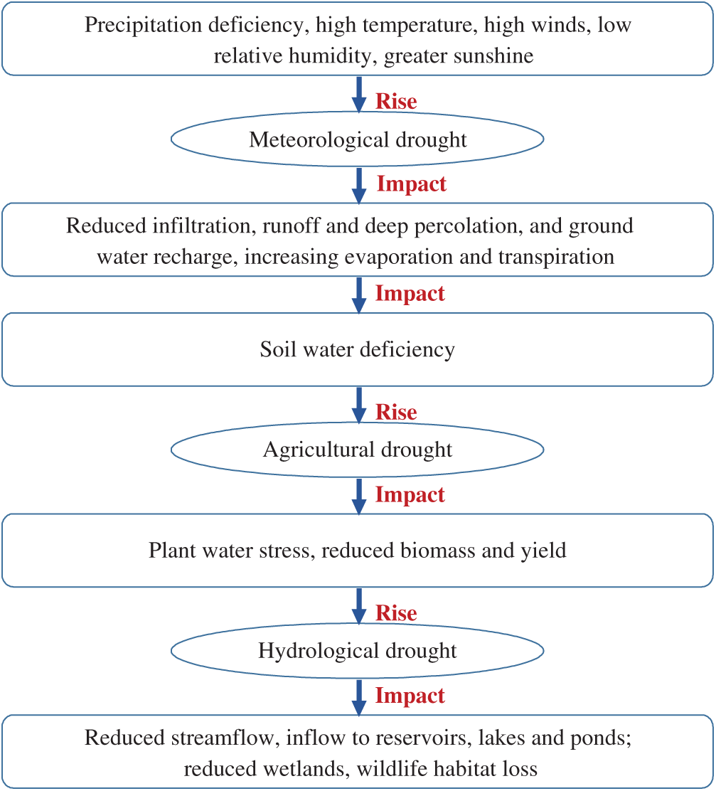
Figure 1: Origin and flow of drought
The impacts of drought differ based on the causes of its origin [5] and include adverse effects on food production, increasing farmers’ suicide rate, excess heat, lower power generation, reduced industrial production, and human and animal health deterioration. In rural areas, it also affects women's security and education. The three main types of impact are economic, environmental, and social impacts.
Plants’ growth depends on the surface and groundwater supplies. It is affected by insufficient water, insect infestation, plant disease, and wind erosion. When the plant's growth is affected, livestock production also gets affected. Farmers lose their income; like a ripple effect, it gets passed on to agro-product retailers and other related business persons. Hence there is a decrease in tax collection of local, state, and central government. It also increases forest fire incidences life-threat to humans and animals.
The damages to the plant and animals will result in a severe environmental impact, including the decrease in water quality and quantity, soil fertility loss, living organisms’ biodiversity loss, and many more. Many species recover from these temporary impacts of drought, but few species become extinct.
There arises a threat to public health and safety. The disputes arising in water resource sharing develop huge rivals between the cities, states, and nations. People start migrating into drought-less places, mainly urban areas. Hence it increases the pressure on the social infrastructure of urban sites.
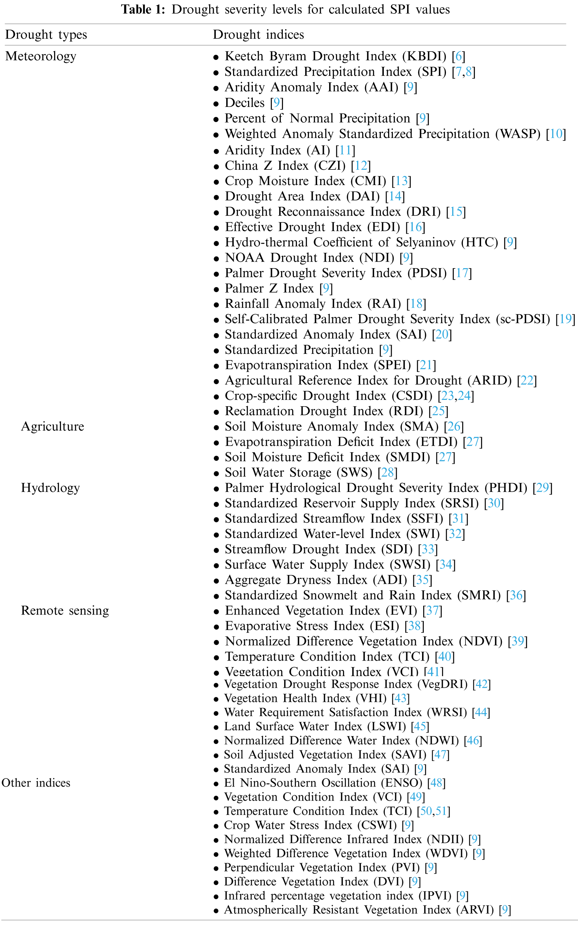
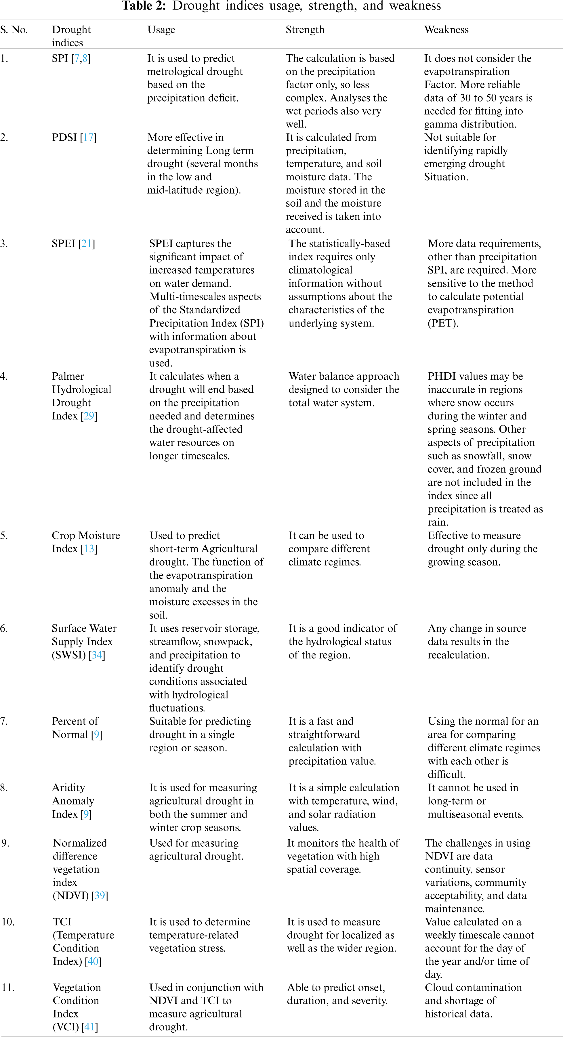
Till now, more than 100 drought indices have been established. These indices help us calculate drought severity, location, start, and end of the drought to help the government issue an early warning to the people and devise contingency plans. Tab. 1 lists various drought indices for predicting different types of droughts. Tab. 2 lists drought indices with their usage, advantages, and disadvantages.
The general temperature increase of about 0.5-degree celsius to 2-degree Celcius is seen in the last 150 years. So the drought indices calculation has also gone through various evolutions. SPEI considered the top most one since it considered the PET in measuring drought severity [52,53]. SRI is needed for measuring socio-economic drought [54]. The aridity index is the opposite of the humidity measure [55]. The software has been created for the calculation of drought indices NDVI [56], PDSI [17,57], Effective Precipitation [58].
There are numerous machine learning (ML)-based predictive modelling techniques used in drought forecasting. There is a need to measure each model's performance and ability to achieve the overall drought forecasting accuracy. The metrics used to assess a model's effectiveness in predicting the outcome is very important since it can influence the conclusion [59]. The performance metrics to identify the error rate between the predicted and observed values are:
• Root Mean Square Error (RMSE) [59]
• Mean Absolute Error (MAE) [59]
• Determination Coefficient (R2) [59]
• The correlation coefficient (r) [60]
• Willmott's Index (WI) [60]
• Nash-Sutcliffe-Efficiency (NSE) [60].
The mean absolute error (MAE) measures the sum of the absolute variation between the forecasted output and the actual output [59]. One cannot identify whether it is underpredicting or overpredicting since all the individual variations have equal weight.
The following equation gives the formula to calculate MAE (Eq. (1)).
where,
N-Represents the total number of data points.
i-Represents a single data from the data points.
Root Mean Squared Error (RMSE) measures the square root of the average squared deviation between the forecasted and actual output [59]. It is used when the error is highly nonlinear. RMSE (Eq. (2)) reports how much error is generated on average concerning the predicted data. It is a good measure of prediction accuracy.
The Determination Coefficient (R2) metric shows the percentage variation in y explained by x-variables, where x and y signify a data set [59]. It finds the likelihood of occurrence of a future event in the predicted outcome (Eq. (3)).
In 1981, Willmott devised an index of agreement (d), which serves as a standardized measure of the degree of model prediction error [60]. The ‘d’ value varies between 0 and 1. The agreement value of 1 indicates a perfect match, and 0 indicates no agreement at all. The additive and proportional differences in the observed and simulated means and variances can be detected (Eq. (4)). However, ‘d’ is overly sensitive to the extreme values due to the squared differences.
where
Nash and Sutcliffe devised the Nash-Sutcliffe Efficiency (NSE) (Eq. (5)) in 1970. Further, it measures the goodness of fit of hydrological models [60]. NSE is a non-dimensional coefficient with a value ranging between −∞ and +1. When NSE =1, then it is a perfect match of the model to the observed data. When NSE = 0, the model predictions are as accurate as the empirical data's mean. When NSE is between infinity (Inf) and 0, that is (Inf < NSE < 0), it is an indication that the observed mean is a better predictor than the model.
3.6 Pearson's Correlation Coefficient
Pearson's correlation coefficient (r) (Eq. (6)) measures the strength of the relationship between two variables’ relative movements [60]. The r-value ranges between −1.0 and 1.0. A correlation of −1.0 shows a perfect negative correlation, while a correlation with a 1.0 value shows a perfect positive correlation. A correlation with a 0.0 value shows no relationship between the movements of the two variables.
where
4 Review on Machine Learning (ML) Methods Used in Drought Forecasting
ML is an application of Artificial Intelligence (AI). ML algorithms are developed with the capability to learn from past experiences and execute new tasks. These algorithms are mainly classified into two categories, namely Supervised Learning and Unsupervised Learning. Supervised learning takes up the labelled data for training and produces a data output from the previous experience. Unsupervised learning is a challenging one, here the system has only the unlabeled data, but it works on its own to discover the information. Fig. 2 shows the taxonomy of the machine algorithms. The Taxonomy of Fig. 2 represents only some of the popular machine learning techniques such as Neural Network, Support Vector Machines, Partial Least Square- Discriminant Analysis, Linear Regression, clustering, expectation-maximization, decision trees, maximum likelihood learning, and Markov process. At the same time, many other machine learning methods such as Deep Learning [61], Fuzzy Logic [62,63], k-Nearest Neighbours, Linear Regression, Singular vector decomposition, and Tenson factorization [64,65], mathematical programming, stochastic modelling, game Theory, phase-type distribution [66,67], semi-Markov modelling [68,69], Gaussian Mixture Modeling [70], discrete-time Markov modelling [71], non-homogeneous Markov modeling [72], Extreme learning machines (ELM) [73] are not included in the figure as there are numerous machine learning methods. It is challenging to have all methods in one figure.
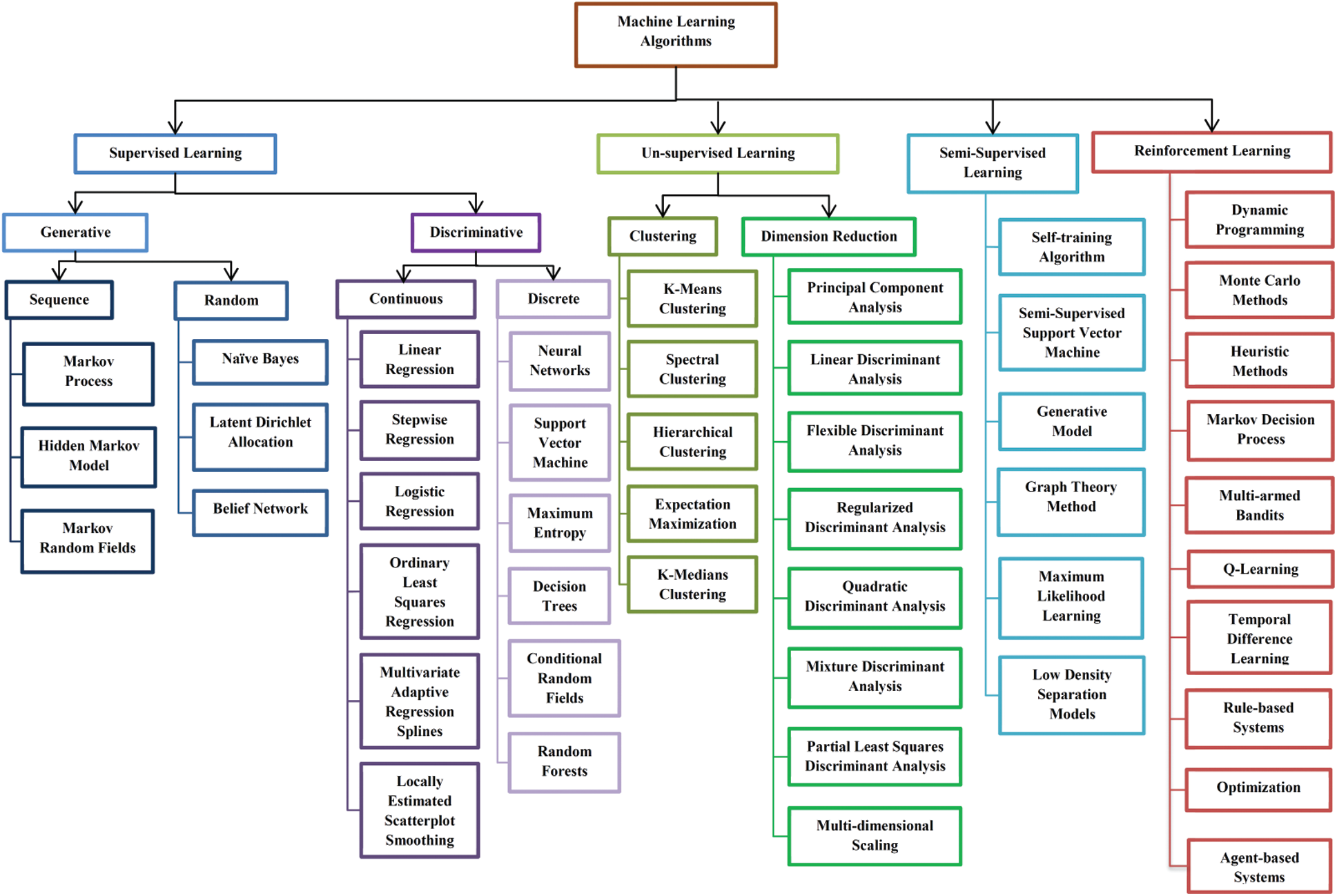
Figure 2: Machine Learning (ML) methods–taxonomy
4.1 A Short View of ML Algorithms Used in Drought Forecasting
Nowadays, Mother Nature is challenging humanity with harsh weather conditions. Natural disasters like floods, hurricanes, and drought are too deadly to sabotage human civilization's prosperity. It takes years and years for us to recover from the fury of nature. The past weather data is a great treasure. So with that past data and ML models, the scientist can achieve 100% accurate weather forecasting. Tab. 3 gives a simple view of the various studies in drought forecasting, describing the ML algorithm used, the dataset used in processing, the area taken for the study, and the drought index used in forecasting. The total number of ML papers considered for review is 83, starting from January 2009 to February 2021. The details of the number of Science Citation Index Expanded (SCIE), Emerging Sources Citation Index (ESCI), and SCOPUS papers are given in the pie-chart shown in Fig. 3.
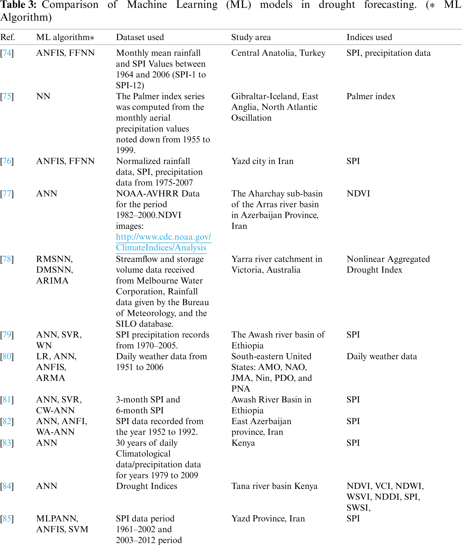
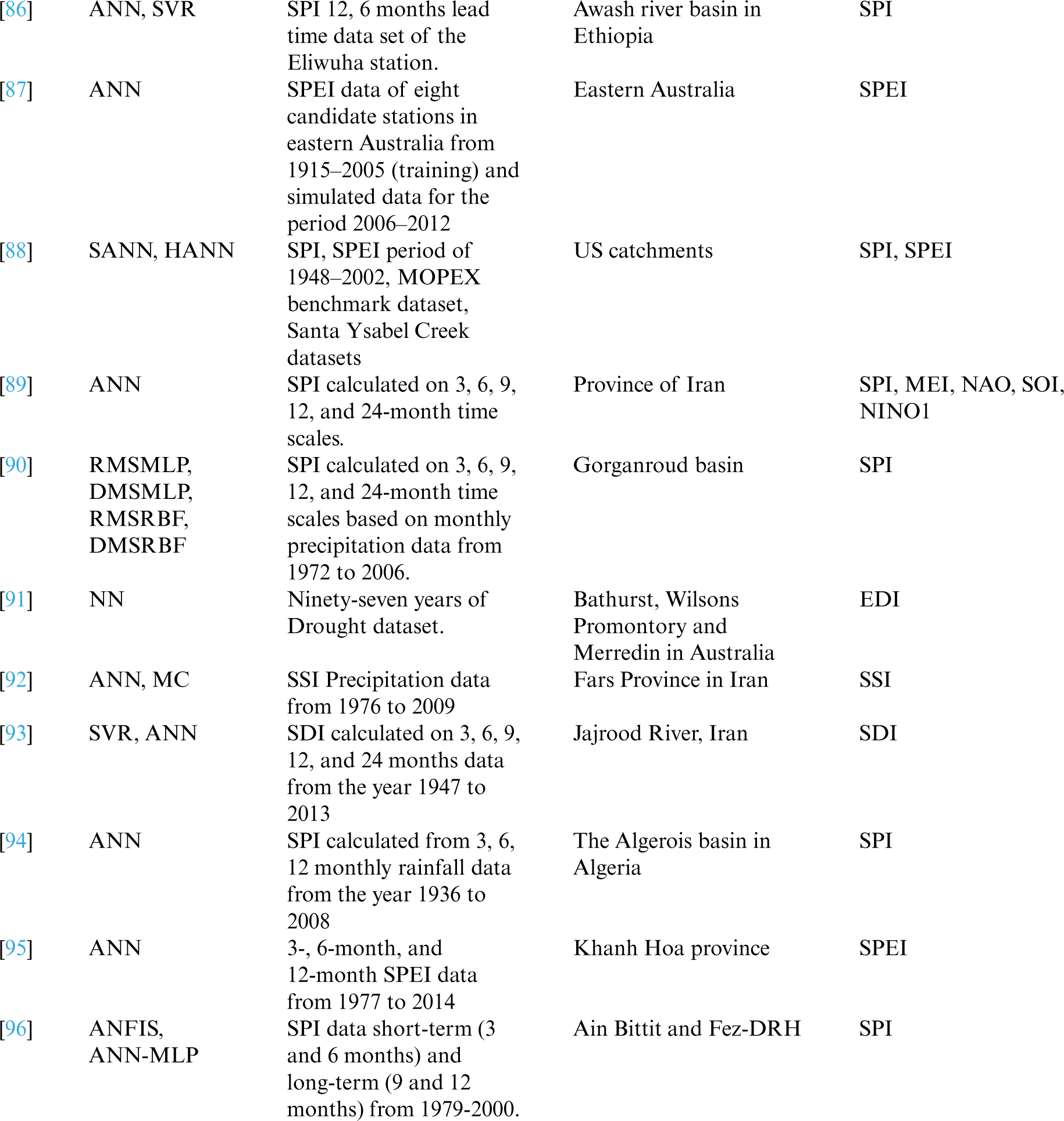
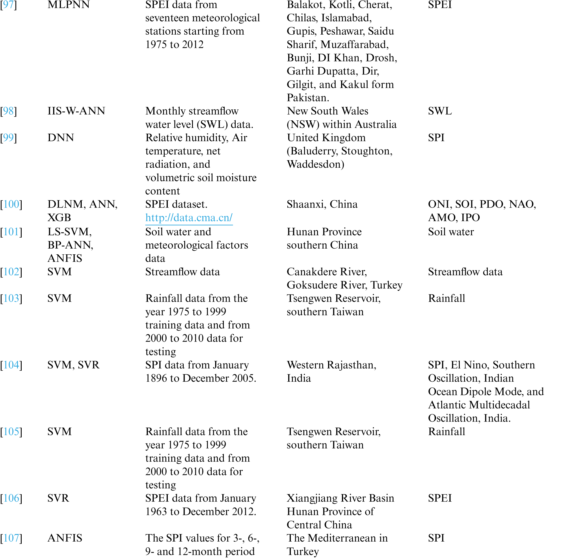
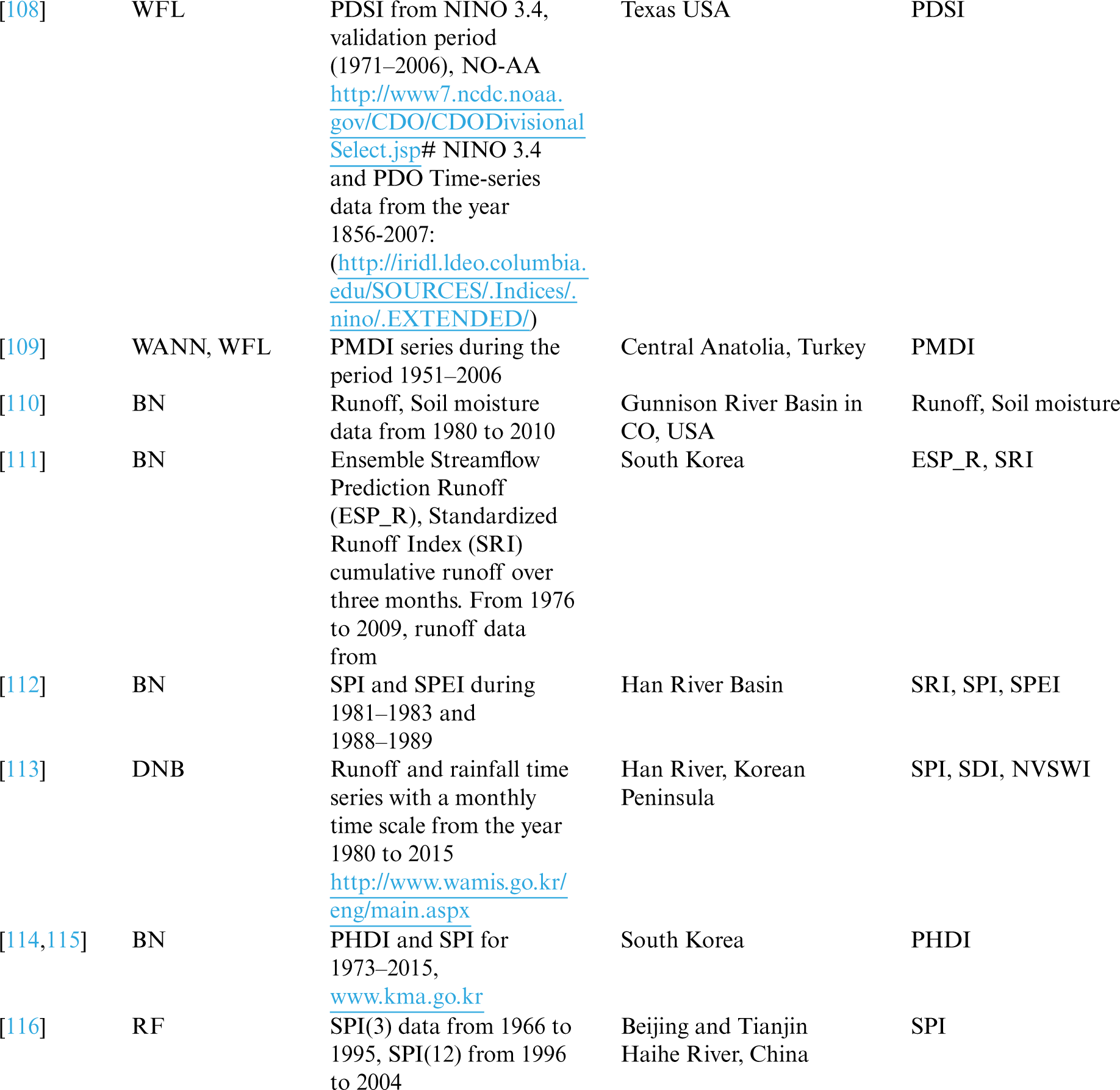
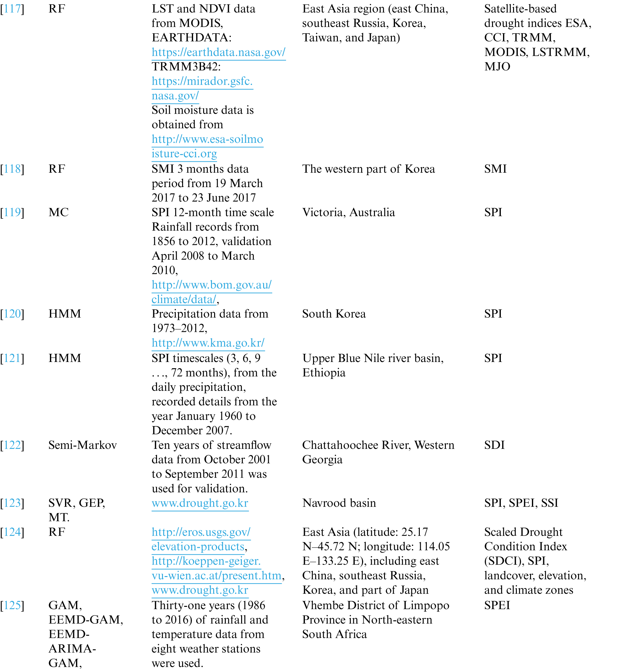
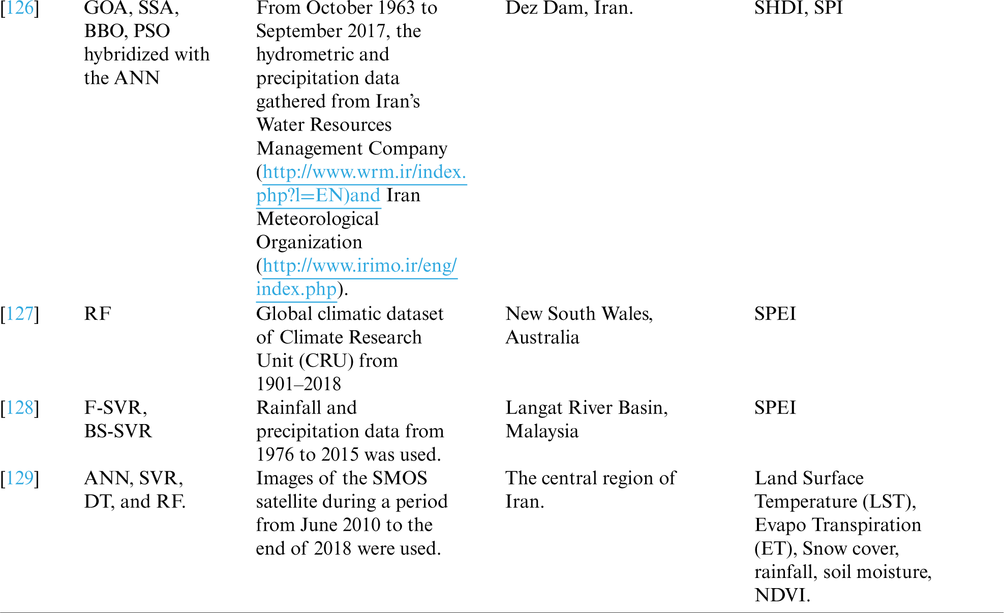
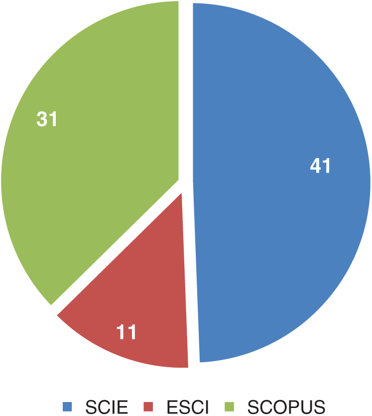
Figure 3: Journal index distribution
4.2 Drought Forecasting Using Artificial Neural Networks (ANN)
Bacanli et al. [74] used the Adaptive Neuro-Fuzzy Inference System (ANFIS) for drought forecasting. The study area taken was Turkey, and the indices used in forecasting were SPI and precipitation. The values from 10 gauging stations of Central Anatolia were taken. ANFIS model was compared with Feed Forward Neural Networks (FFNN) and Multiple Linear Regression (MLR). It has been found that the Adaptive Neuro-Fuzzy Inference System (ANFIS) provides higher accuracy and reliability.
Dastorani et al. [76] developed a model to predict the precipitation value-12 months in advance. The precipitation prediction was made for Yazd, Iran. Three models were developed-Recurrent Network (RN), Time Lagged Recurrent Network (TLRN), and ANFIS. The parameters taken were wind speed, wind direction, relative humidity, maximum temperature, normalized rainfall data, seasonal and 3-month average precipitation, and mean temperature for the period 1975 to 2007 for ANFIS five-layer processing was done. The results showed that among the ANN models, TLRN prediction accuracy was very high. They compared the prediction accuracy of TLRN with ANFIS, and it was found that both the methods performed equally well. A new fact found was, when 3-year moving average precipitation was added to the input, best results were achieved, in which case, ANFIS was predicting better than TLRN.
Marj et al. [77] predicted the agricultural drought in the Aharchay Basin in Azerbaijan Province in Iran's northwest. Further, they used the NDVI values with two climatic signals in the ANN model for prediction. The two climatic signals used were the SOI and NAO. From the NDVI, the Anomaly Vegetation Index (AVI) and Vegetation Condition Index (VCI) were calculated. The three months viz. May, June, and July data from 1982 to 1999 were used to train and test the model. May, June and July were agricultural months considered for the study. The results showed that the standard deviation for predicted and observed NDVI was less than 1. This study also suggested a low correlation between the rainfall recorded and NDVI values predicted in this area.
Belayneh et al. [79] selected an area with drastic climatic variations year by year. The chosen site was the Awash River Basin of Ethiopia. Since there was a significant difference in this area's climate, it was divided into Upper Awash Basin and Lower Awash Basin. Three data-driven models were developed for predicting SPI value-ANN, Support Vector Regression (SVR), and Wavelet Neural-networks (WNN). The three models’ performance was compared using MAE, RMSE, and R2 performance values. The WNN provided a better SPI prediction in all three basin areas. All the models showed greater accuracy in determining SPI 12 than SPI 3.
Masinde et al. [83] used ANN to predict the Effective Drought Index (EDI). The study was carried out in Kenya, where rainfall was the only source for agriculture. With the help of 30 years of data from four network stations, the ANN model was developed. Kenya Metrological Department used statistical techniques to predict the rainfall probability as normal, above average, and below average. With these values, one can get only the conceptual indication of drought. However, ANN was deployed to forecast the drought starting period, severity, and duration of drought. EDI is an excellent drought indicator. First, the EDI was calculated using the following procedure. The Java code was used to clean and format the 30 years’ data. Subsequently, this data was processed by the EDI Fortran program. Then, the ANN model was constructed. The ANN used the EDI, precipitation, and AWRI values for the years 1980 to 2009. Lead time for a day, month, and year forecast outputs were obtained. The experimental results showed the day lead time forecast with precipitation and provided an accuracy of 98%.
Hosseini-Moghari et al. [90] aimed to compare direct multi-step neural networks’ performance and recursive multi-step neural networks. The MLP, RBF, and GRNN neural networks were taken for the study. The overall results obtained inferred that the RBF shows good accuracy, followed by MLP and GRNN.
Belayneh et al. [81] were the first to experiment with coupled ML methods and ensembling techniques in drought forecasting. Wavelet transformation was applied to ANN and SVR. In wavelet analysis, the original time series was modified into a new time series. A wavelet was used to denoise the time series data, and WANN and WSVR were created. The k-fold bootstrap validation technique was used to construct BANN and BSVR. With the ensembling of boosting methods, BSANN and BSSVR were created. SPI 3, SPI 12, and SPI 24 predictions were accomplished using the models mentioned above for forecasting the meteorological drought. The performance comparison among the models was accomplished using RMSE, MAE, and R2.
Prasad et al. [98] integrated the wavelet hybrid ANN with an Iterative Input selection algorithm (IIS) to forecast the streamflow in Australia's Murray-Darling basin to plan water utilization and redistribution. The new model was the non-decimated Maximum Overlap Discrete Wavelet Transform (MODWT) algorithm using ANN as a primary model. M5 model was used as the benchmark evaluation. IIS was used to select the best predictors since there were many predictors like maximum and minimum temperature, precipitation, solar radiation, vapour pressure, and evaporation.
Zhang et al. [100] carried out SPEI prediction in the Shaanxi province of China. Totally three procedures-ANN, DLNM, and XGBoost models were implemented and compared. SPEI 3, SPEI 6, SPEI 9, and SPEI 12 were predicted using the data from 1961 to 2016 with a 1 to 6 months lead time. The results showed that the XGBoost method showed better accuracy than the other two predicting the widespread drought and drought category.
Kisi et al. [130] accomplished the SPI prediction using classic ANFIS and conjunctive ANFIS models embedded with meta-heuristic optimization algorithms, namely particle swarm optimization (PSO), Genetic Algorithm (GA), Ant colony Algorithm (ACO), and Butterfly Optimization Algorithm (BOA). SPI-3, SPI-6, SPI-9, and SPI-12 prediction for the three stations in Iran's Semnan Province were performed. Evolutionary algorithms outperformed classic ANFIS performance in all the stations and for all SPI values prediction. The performance of ANFIS-PSO was outstanding than the other three methods.
Mulualem et al. [131] determined the climatic indicators that better calculate SPEI. The study used the 30 years of data from 1986 to 2015 for Ethiopia's Upper Blue Nile Basin. Totally seven ANN models were designed for predicting SPEI by incorporating the factors like hydro-meteorological, climate, sea surface temperatures, and topographic attributes to forecast the SPEI. Totally 12 climatic indicators were taken, and their various combinations were fed into the seven ANN models. The three climatic indicators, maximum temperature, evapotranspiration, and rainfall, were found to be prominent.
Moazenzadeh et al. [132] predicted the evaporation factor. This factor was not measured in most of the metrological stations. However, this factor seemed to be essential for determining the water resource share. The evaporation factor was predicted at two meteorological stations (Rasht and Lahijan) located in Gilan province in northern Iran using SVR and SVR coupled with Firefly. The Pearson correlation coefficient was used in identifying the parameters which had more impact on evaporation prediction. The selected parameters were the maximum air temperature, net solar radiation, mean relative humidity, wind speed, precipitation, sunshine hours, and saturation vapour pressure deficit. Seven parameters were taken, but SVR and SVR-FA prediction reached the best when a more significant number of inputs were used.
Streamflow Drought Index (SDI) was introduced in 2008 by Nalbantis [133]. Further, this was used to calculate the intensity, duration of drought, for which it needs monthly discharge data. Woli et al. [80] devised methods to forecast SDI using SVR and ANN and studied the best input combinations used in forecasting. The Pearson coefficient of type III was the best statistical for each time scale of monthly discharge intervals of 3, 6, 9, 12, and 24. The gamma test was used in finding the input combination. The SDI was predicted in 3, 6, 9, 12, and 24 month periods for using the corresponding delays of SDIt, SDIt-1, SDIt−2, SDIt−3, and SDIt−4 as the primary inputs and SDIt + 1 as the target variable. Results were taken with all inputs first and then by leaving the input variables one by one. The gamma test found that SDIt (no delay) and SDIt−1 (1-month delay) had a high impact on the forecast.
Alsumaiei et al. [134] established the Nonlinear Autoregressive Networks (NAR), a unique type of Recurrent Neural Network with the combination of ANN and autoregressive models used to describe processes based on lagged input and output variables for predicting precipitation index. The correlogram test was conducted on the observed precipitation index time series to evaluate adjacent values’ correlation and predict the next time step value. NAR was found to be a reliable model for drought forecasting.
4.3 Drought Forecasting Using Support Vector Machine
Ganguli et al. [104] tried the ensemble Support Vector Machine (SVR) with Coupla for predicting metrological drought in Rajasthan. The Least Square SVR model was used in drought index forecasting. Bivariate Coupla functions were used to model the uncertainty associated with drought forecasting. Three types of copulas, namely the Frank, Clayton, and Plackett families, were taken to study drought forecasting. Forecasting was done up to a three-month lead time. From the experimental results, it was found that the prediction performance increased when climatic indices were added.
Chiang et al. [105] established the two-stage SVM model for reservoir drought forecasting. First, the single-stage SVM was devised, and then it was compared with the other three models. The 90 days lead time forecast achieved up to 80% accuracy. Both studies forecasted the reservoir drought for the Tsengwen reservoir, the largest reservoir in Southern Taiwan. In a two-stage SVM, four parameters were used as input. They were reservoir storage, inflows, the critical limit of operation rule curves, and the Nth ten-day in a year. The training data was from 1975 to 1991, and the testing data was from 2000 to 2010. In the first stage of the SVM, drought or non-drought was predicted. In the second stage of SVM, the drought category was predicted as Drought or Severe Drought. The LIBSVM tool was used in the implementation, and the results were compared with Artificial Neural Networks (ANN), Maximum Likelihood Classifier (MLC), and Bayes classifier (BC). The SVM model outperformed the other three models in predicting the non-drought category and its ten-day predictions were above 90%.
Kisi et al. [102] framed a model to forecast the monthly streamflow in Gerdelli Station on Canakdere River and Isakoy Station on Goksudere River in Turkey's Eastern Black Sea region. The model was constructed by combining discrete wavelet transform and support vector machine; the past data's time-series were decomposed into three sub-time series components (D1, D2, and D3) by the Mallat DWT algorithm. D1, D2, and D3 represent the time series mode of 2 months, 4-months, and 8-months, respectively. RMSE, MAE, and R were the performance metrics evaluating WSVR with SVR model accuracies. Totally 40 years of observed data for both stations were collected. Out of this, 75% was used for training and 25% for testing. The output showed that the WSVR conjunction model increased the prediction correlation coefficient concerning the single SVR model by 19%–30%. There was a reduction in the root mean square errors and mean absolute errors by 11%–46% and 19%–44%.
Memarian et al. [135] determined the Co-Active Neuro-Fuzzy Inference System (CANFIS) capability for drought forecasting of Birjand, Iran. The various global climatic signals were explored in addition to the rainfall and precipitation. In total, nine climatic signals were used. NINO 1 + 2 describes ocean level temperature; NINO 3 and NINO 3.4 describe the Pacific Ocean's surface temperature. Tropical Southern Atlantic index (TSA) measures the Atlantis surface temperature. SOI was based on water surface pressure. NAO index was calculated using pressure fluctuations in the North Atlantic Ocean. Based on the beach's average monthly precipitation for Arizona and New Mexico regions, SW Monsoon Region Rainfall (SWMRR) was measured. Multivariate ENSO Index (MEI) was calculated using the parameters such as water surface pressure, temperature, and wind velocity. Thermal fluctuations of the Atlantic Ocean were used in measuring Atlantic Multi-decadal Oscillation (AMO) index. The neural network and fuzzy rules were combined, and the neuro-fuzzy structure was formed. CANFIS performs well in index NINO 1 + 2 with five months lag.
Djerbouai et al. [94] investigated ANN and Wavelet ANN's prediction accuracy against the stochastic models ARIMA and SARIMA. The difference between ARIMA and SARIMA was that the ARIMA worked well with static data, and SARIMA also functioned with non-stationary data. SARIMA was a non-seasonal model used in modelling seasonal time series with varying mean and other statistics across the years. The experimental results showed that the SPI-12 model provided good forecast than SPI-3 and SPI-6 in one-month lead prediction.
Tufaner et al. [136] preferred the regression methods, and the selected input variables had shown promising results. The metrological variables were used as input data. Among the classification techniques ANN, Decision Tree, and SVM, ANN had a correlation coefficient of 0.98.
4.4 Drought Forecasting Using Fuzzy Logic
Shirmohammadi et al. [82] developed drought forecasting using wavelet ANN and ANFIS methods with SPI. The metrological drought was tested at different time scales. The study site selected was Tabriz, East Azerbaijan province, Iran; the data period 1952 to 1992 was used to test and then predict the meteorological drought test period extending from 1992 to 2011. Further, to build this hybrid model, the sub-series data played a significant role. In step 1, the original SPI data were decomposed into details using discrete wavelet transform. By applying successive approximation signals, the decomposition process was iterated, and hence the original time series was broken down into lower resolution components of levels 1, 2, 3, and 4. Seven different kinds of wavelets, namely, db4, bior1.1, bior1.5, rboi1.1, rboi1.5, coif2, and coif4 wavelets, were used. Out of the four models ANN, ANFIS, wavelet ANN, and wavelet ANFIS, wavelet ANFIS produced good prediction accuracy. Woli et al. [80] explored the use of climate indices like ENSO as a predictor. The ARID index was based on ENSO, and its efficiency in drought forecasting was studied. The ARID index with four methods was predicted: ANN, ANFIS, LR, and SARIMA models. The climatic indices, namely JMA, AMO, NAO, Nino-3.4, PDO, and PNA, were deployed. During winter, the ENSO signals were strong, and hence LR and ANFIS prediction were higher. SARIMA model provided the correct prediction in the months where the precipitation was high. However, ANN offered the overall best prediction performance from March to December.
Ozger et al. [108] concentrated on finding the PDSI values for drought forecasting. For PDSI calculation, precipitation, temperature, soil moisture, and previous PDSI values were needed. They witnessed that obtaining past year data for precipitation and temperature was easy, but it was challenging for them to get the soil moisture values. The Wavelet Fuzzy Logic (WFL) was used to predict the PDSI. It was found that temperature and precipitation predictors give the best results in predicting PDSI values. Agboola et al. [137] made rainfall prediction in Nigeria using Fuzzy logic. The fuzzy logic model contained two components. The first component was the knowledge base, where the if-then rules with decision making were made. The second component was the decision unit, performing inference operation. The input variables used were temperature, pressure, humidity, dew point, and wind speed. The error rate was very minimal. Hence, it was proved that the Fuzzy logic could be used in the rainfall prediction of Nigeria.
Shin et al. [114] designed a model, namely Bayesian Networks based Drought forecasting with Drought Propagation (BNDF_DP), which incorporates dynamic model predictions and a drought propagation relationship. The basic idea used was the drought persistence and transition properties in the drought. The metrological drought occurs initially due to the lack of precipitation followed by a reduction in soil moisture and groundwater depletion. It leads to agricultural drought and hydrological drought. The conversion period from meteorological drought to hydrological drought is called lag time. The hydrological drought forecasting was made using the PHDI and the SPI. The model was constructed with three-parent nodes, namely HDn-current hydrological condition, MHDn+l-predicted hydrological drought using Asia-Pacific Climate Center Multi-Model Ensemble (APCC MME) forecast, SPIn+l−lt; l–lead-time and lt-lag-time) and one child node (HDn+l). ROC Curve analysis proves the proposed model's superior forecasting skills for long-term drought, with a 2 and 3 month lead time. Sattar et al. [112] attempted to trace the probability of hydrological drought in Korea's Han River. The Bayesian model finds the probabilistic relationship of weekly lag time between hydrological drought and metrological drought.
SPI and SPEI values define the metrological drought, and SRI describes the hydrological drought. Out of 24 sub-basins of the Han River, four sub-basins were chosen for the study. The daily records of precipitation were collected from the Korean Metrological department. From the precipitation data, the evapotranspiration and runoff were calculated using the TANK model. A metric called Response-rate gives the percentage of metrological drought converted to hydrological drought. The joint probability between the lag time and drought Intensity, P(I, LT), was estimated using a Coupla function. Four Coupla functions were examined, namely, Gaussian, T, Gumbel, and Clayton. Further, the Gaussian was chosen as the best choice. Bae et al. [111] devised a Bayesian model-based approach to find the hydrological drought using. The posterior distribution was found out using the Bayesian model using the prior distribution regression result between Historical Runoff (HR) and Ensemble Streamflow Prediction Runoff (ESP_R) as the prior information and a conditional equation derived from the linear regression model as a likelihood function.
Mehr et al. [138] developed a novel fuzzy random forest (FRF) model to predict SPEI. The dataset was divided into smaller subsets/branches similar to the divide and conquer algorithm until the branch shows the class directly. An ensemble of FRF overcame the inefficiency of the Fuzzy decision Tree in handling nonlinear data.
4.5 Drought Forecasting Using Markov Chain (MC) Model
Aviles et al. [139] pointed out the impacts of the drought condition in the Andean mountains of south Ecuador using the reinforcement learning-based MC model and Bayesian Network (BN) method. Out of the four Coupla functions, two elliptical and two archimedean, the best was estimated using the parametric bootstrap-based goodness-of-fit test. The Ranked Probability Skill Score (RPSS) was used to evaluate the performance of the models. The results showed that the BN-based models were better at predicting severe drought events than the MC-based models. Khadr [121] developed various Hidden Markov Models (HMM) using SPI to predict the drought. The HMM's speciality is that the output is conditionally independent, which helps us understand the local scale statistics at a larger scale. The HMM performed well with a short lead time, but the forecast accuracy decreased once the lead time increased. HMM performed well for a lead time of 7 months. Shuang et al. [140] devised the hybrid hidden Markov model coupled with multivariate copula for metrological drought forecast with SPI time series. With Bayesian Inference, the model structure and parameters were optimized. The mixture distribution for each prediction was a weighted combination of posterior copula conditional distributions. Further, they also concluded that this method is more accurate than ANN, ARMA, and HMM.
4.6 Drought Forecasting Using Deep Learning
Agana et al. [141] created a hybrid predictive model using a denoised empirical mode decomposition (EMD) and a deep belief network (DBN). The StreamFlow Index (SFI) was predicted. The strength of EMD is decomposing any complicated dataset into a finite number of Intrinsic Mode Functions (IMF) of different dominant frequencies and amplitudes. Selecting the IMF is done by Detrended fluctuation analysis. EMD servers were better in input decomposition than wavelet analysis. Chen et al. [142] framed the Deep Belief Network (DBN) based model and compared it with Backpropagation Neural Network; it was observed that DBN was more reliable and efficient for short-term prediction of drought index. SPI12, SPI9, SPI6, and SPI3 predictions were made. The RMSE and MAE values get minimized with the increase in SPI timescale. The RMSE value in the range of 0.4 to 0.5, and the MAE value in the range of 0.2.to 0.3 was achieved in study stations. Poornima et al. [143] utilized a correlation coefficient test to determine the climate indicator along with SPI, SPEI prediction. Long short-term memory was used in a recurrent neural network to predict the drought indices. Zhu et al. [144] worked on the aggregation of LSTM with the Conditional Probability Model (CPM), namely Gaussian Process Regression (GPR). Thess models were accomplished in two various forms by GPR-LSTM-S1 and GP-LSTM-S2. In GP-LSTM-S1, the GPR was used for analyzing the forecasting error series, and in GPR-LSTM-S2, the GPR was embedded in the last hidden layer. GPLSTM-S1 lacks performance stability as compared with GPLSTM-S2. Further, they concluded that the LSTM was good at handling the high-dimensional data.
The most important findings observed in the study in this paper are discussed in various sections. In Section 5.1, the results related to multiple ML processes are given. The finding on the hydrological drought prediction is given in 5.2, and 5.3 discusses future work.
5.1 Review Findings Based on ML Model
The critical observation found from the papers taken in this review related to the ML algorithm's five primary processes, namely Data Collection, Feature Selection, prediction model construction, ensembling, performance evaluation, and parameter tuning, are given below.
5.1.1 Data Collection and Preparation
The accuracy of any machine algorithm depends primarily on the quantity and quality of data. In this phase, the necessary data collection was accomplished. From the extensive collection of nearly 75 years of precipitation, rainfall, and temperature data, many drought indices like SPI, SPEI, and PDSI are derived. From the literature reviewed in this paper, we can see that the SPI, SPEI, PDSI, NINO, ELINO data are predominantly used. New Drought indices are used by subjecting the available water-related variables to PCA, calculating the correlation matrices between time series ‘r’ and available hydro metrological datasets, yielding the Eigenvalue Eigenvector. Mulualem et al. [131] determined the climatic indicators that calculate the best SPEI. It was found that the best indices for SPEI prediction were rainfall, maximum temperature, and evapotranspiration. Ozger et al. [108] proved that the PDSI prediction with WFL requires temperature and precipitation data predominantly. Borji et al. [93] obtained a virtuous result in SDI prediction with the Gamma test. Marj et al. [77] proved a low correlation between the rainfall recorded and NDVI values predicted. They also forecasted NDVI using two climatic signals NAO and SOI, recorded in the preceding spring. Mehr et al. [109] performed the sensitivity analysis among input variable bands and found the impact of the initial values of PMDI on predicting drought within a 6-month lead-time. NIÑO 3.4 had a high potential to forecast drought for 6-through 12-month lead-time. There was a need for cleaning the data received from weather stations. Most of the data in past years were stored in the format used by FORTRAN. It needs to be transformed into the required format for further processing by the machine learning models.
Ali et al. [145,146] decomposed 12 input predictors into nearly 120 sub-components. Simulated Annealing was used to choose the most appropriate IMF's for the training period. KRR was used to forecast the multiscalar SPI series. The solution was designed to use dynamically driven climatological factors such as atmospheric circulation instead of univariate data. Dikshit et al. [147] SPEI forecasting was good in predicting drought since it considers both the temperature and rainfall. The atmospheric and oceanic phenomena were considered, but it was found that the sea surface temperature does not have much significance. Han et al. [148] suggested using remote sensing data in gauge scarcity areas. Since it was prone to systematic bias, they merged it with the in-situ data. Bojang et al. [149] stated that Single Spectrum Analysis (SSA) is an all-time best time series analysis method. It can be customized to any underlying dataset, and it does not need any prior modelling. Hence, they termed it as a model-free method. Decomposition and reconstruction is the two process in SSA. The decomposition is done by performing embedding and singular value decomposition. Han et al. [148] aimed to synthesize the forecasting models used in drought forecasting and tree mortality based on causative mechanisms and global warming implications. For better forecasting, the statistical models with nonlinear and non-stationary behaviour have to be merged with dynamic models to improve their stochastic characteristics. Fig. 4 shows the indices and number of papers used in this review paper.
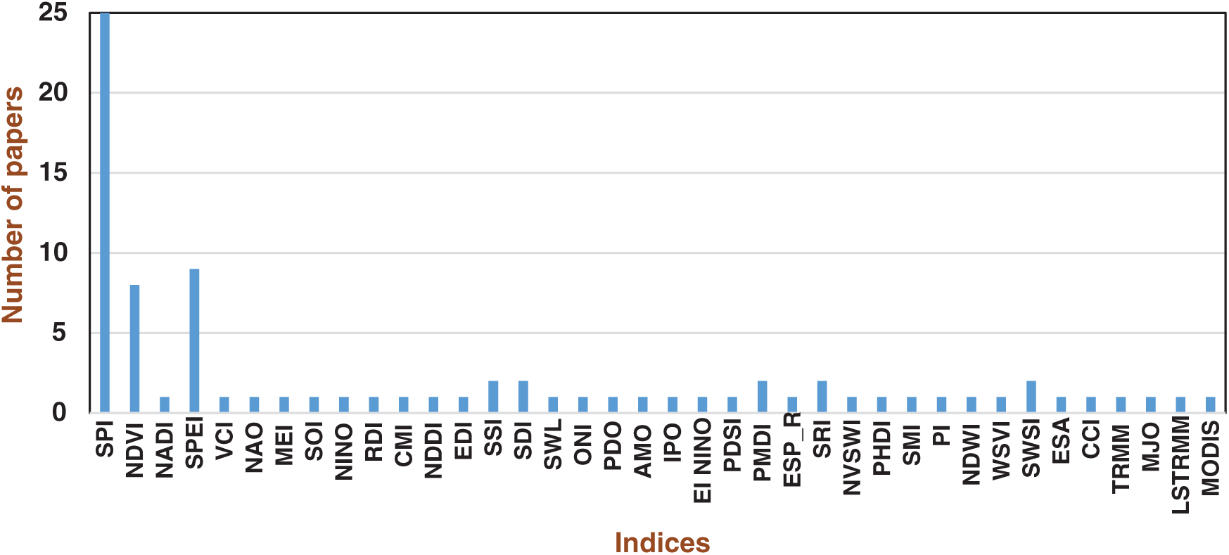
Figure 4: Drought indices vs. number of papers
The input for the drought prediction models was given as processed data. The calculated time series data of drought indices get transformed into new time series data. Wavelet analysis helps to de-noise a particular data set; the transformation from the original time series to the new time series was done using wavelet analysis and was used as an input. The appropriate input combination to be fed into the model was pre-processed using the gamma test [93]. Many ML studies proved that feature selection improves classification accuracy and reduces processing time. A tree-based iterative input selection (IIS) algorithm was used to test and sort a global predictor matrix. Through a Copula-based approach, the ensembles of drought indices were determined [104]. In NDVI values, the selection of the proper cells within the SST and SLP databases was done by linkage data mining models and using the geographical information system (GIS). Probability distribution fits the precipitation data of each station to identify observed precipitation probabilities. The appropriateness of normal and exponential probability distributions was examined by the Kolmogorov-Smirnov (K-S) test. Deng et al. [101] performed data denoising by heursure and rigrsure algorithms, with bior3.3 associated with biorthogonal wavelets with three decomposition levels. Zhang et al. [100] found that more period was needed when many predictors were used. Mehr et al. [109] also proved that using the wavelet algorithm minimizes the noise, and it helped well in PDMI prediction using LGP. Genetic Algorithm is used in optimizing the weights of ANN. Using PCA (Principle Component Analysis) the 9 different drought attributes is reduced to 4, to improve classification and reduce time [150].
Dastorani et al. [76] found a new fact that, when 3-year moving average precipitation was added to the input, the best results were achieved. Farokhnia et al. [151] witnessed that SST and SLP data's application improved the ANFIS model's performance. Shirmohammadi et al. [82] determined that the wavelet transforms better handle nonlinear and non-seasonal data.
5.1.3 Building the Drought Prediction Model
Many ML models are available for building the drought prediction model. Many successful studies used various ML techniques for drought prediction. The most commonly used ML models are ANN-based, fuzzy, SVM, Bayesian, Random forest, and many more. Generally, the ANFIS offered a better prediction than TLRN [76] with 3-month average precipitation. Fig. 5 shows the ML models used in drought prediction vs. the number of papers.
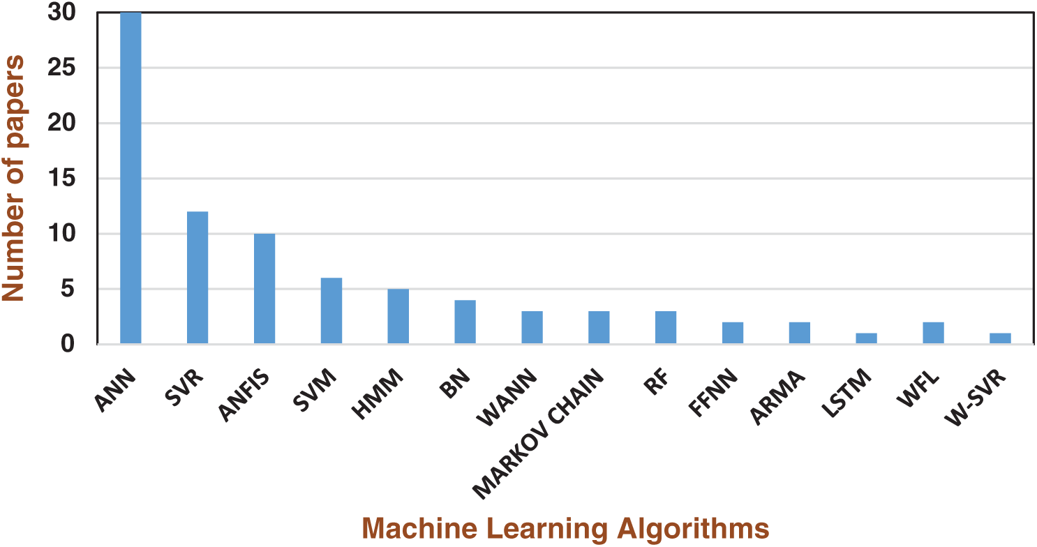
Figure 5: Machine Learning (ML) algorithms vs. the number of papers
5.1.4 Ensembling of ML Algorithms
Two heads can perform better than one; similarly, when more than one ML model is used in prediction, it will improve the accuracy. The bootstrap technique can be applied by creating bootstrap ANN and SVR ensemble models. Ibrahimi et al. [96] showed good SPI prediction using WANFIS than WASVR and WAANN MLP models. Finally, the results predicted that wavelets boosted ANN and SVR-WBSANN and WBSSVR had better forecasts than other models. Djerbouai et al. [94] clearly explained that the wavelet ANN and wavelet ANFIS wavelet models could cope with the nonlinearity and variations in data due to seasonal changes. Zhang et al. [100] proved that extreme gradients with linear booster performed well. Khan et al. [152] established the metrological drought indices such as the Standardized Precipitation Index (SPI) and the Standard Index of Annual Precipitation (SIAP) values. These values were decomposed into low and high-frequency sub-series by Discrete Wavelet Transform, and then it was passed on to the predictive models of ARIMA and ANN. The wavelet-based ANN had achieved a correlation coefficient value of 0.41 for SPI prediction. The hybrid wavelet-ARIMA-ANN models gave the R2 value of 0.872 for SPI. Malik et al. [153] used Effective Drought Index to predict metrological drought using the heuristic techniques, namely, the co-active neuro-fuzzy inference system (CANFIS), multi-layer perceptron neural network (MLPNN), and multiple linear regression (MLR). The monthly time series data lag was determined using the autocorrelation function and the partial autocorrelation function. The hybrid ANFIS algorithm's performance was better than the classic ANFIS algorithm. Mohamadi et al. [154] captured the relationship between large-scale climate signals and drought indices using a wavelet coherence analysis. Hybrid soft computing models and wavelet coherence seem to be the appropriate tools for predicting hydrological variables.
5.1.5 Evaluating Our Model and Parameter Tuning
The performance of the classification algorithm is measured using various evaluation metrics. This feedback on the model is needed to fine-tune the model by varying the algorithm's parameters. The most commonly used performance measures are RMSE, R2, MAE, NSE, RPSS, and ROC. Mehr et al. [138] evaluated the forecasting model using Boolean statistics, namely total accuracy (TA), Kappa (KA), recall (RE), and classification error (CE).
Fig. 6 gives the details of the performance evaluation metrics and the number of papers using them.
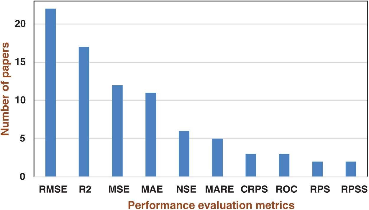
Figure 6: Performance evaluation metrics vs. number of papers
The gradient descent and least square methods were used to tune the antecedent and consequent parameters in the ANFIS model. The gradient descent method was used to assign the nonlinear antecedent parameters, and the Least-squares method was employed to identify the linear consequent parameter. The number of iterations taken for the correction of the model parameter was 30 [80]. All coefficients of the linear membership function were estimated using the Least Square Technique from the datasets. Using the Bayesian regularization (BR) [74], ANN automatically assigned the optimum values for the objective function's parameters.
5.2 Findings on Hydrological Drought Forecasting
Sattar et al. [112] discovered the probabilistic relationships between the meteorological droughts intensity and lag time. There was a higher probability for longer lag time for moderate intensity, whereas there was a lower probability of longer lag time for severe intensity. The Meteorological drought indices, at the same intensity, also impacted the probability of lag time. The probability of lag time occurring was higher in SPI and lowered in the case of SPEI. Using ESP and metrological drought data, the Bayesian model found the hydrological data more accurate than ESP and Dynamic methods. So et al. [155] Modified Surface Water Supply Index (MSWSI) was used as an index in hydrological drought forecasting. The topographical and hydro-meteorological characteristics of South Korea were used. Further, this work depicted the hydrological drought better by using precipitation, river discharge, and dam inflow during 3-month periods. Global Seasonal Forecast System version 5 (GloSea5) and variable infiltration capacity (VIC) model was used in the forecasting framework, and the testing was done for the 2015-16 drought event.
5.3 Drawbacks of ML Algorithms
A massive amount of historical data is needed to train and develop the ML model. The data unavailability will reduce prediction accuracy. The challenges are the need for high-resolution images without cloud contamination for the models collecting the data from satellite images. Supercomputers are required for the weather forecasting process. The earth is a vast, complex system. Hence it requires a high-resolution monitoring system.
Prasad et al. [98] suggested deploying an IIS-W-ANN optimization algorithm for drought forecasting. Further, they suggested that this model's performance could be improved by fine-tuning the hidden layer weights and biases. Ozger et al. [108] suggested that future researchers should work on the estimation of soil moisture from PDSI. Mehr et al. [109] devised a model to determine the drought using other climatic indices and analyzed the effect of various wavelet functions in optimizing the model. Kisi et al. [102] also suggested working with other DWT algorithms like the Trous algorithm for enhanced drought forecasting. Borji et al. [93] suggested using a genetic algorithm and multiple regression in pre-processing. Further, it was stated that the detected SST/SLP cells [129] are a future study area to investigate other climate events’ impact. Woli et al. [80] established the use of climate indices as a predictor. Ali et al. [146] studied monthly SPI prediction for three agricultural stations of Pakistan using the committee-based extreme learning machine (ELM) and insisted on future researchers working on an adaptable decisions support model.
Dikshit et al. [147] had pointed out that a detailed study on the effect of variables on the spatial scale is needed. Khan et al. [152] suggested studying the application of coupled wavelet-ANN-ARIMA models for hydrological drought prediction with different lead times is required.
This paper's extensive literature review found that the drought indices used in prediction and ML algorithms applied are the primal factors in drought prediction. An archetypal portrayal of the ML-based operational model for drought forecasting is shown in Fig. 7. Further, this figure demonstrates various constituents that aids in improving the performance of attaining precise drought forecasting outcomes. A single classifier was used in most articles, and the multiple or hybrid classifier usage looks minimum. Also, the usage of multiple drought indices for prediction seems to be a practical solution.
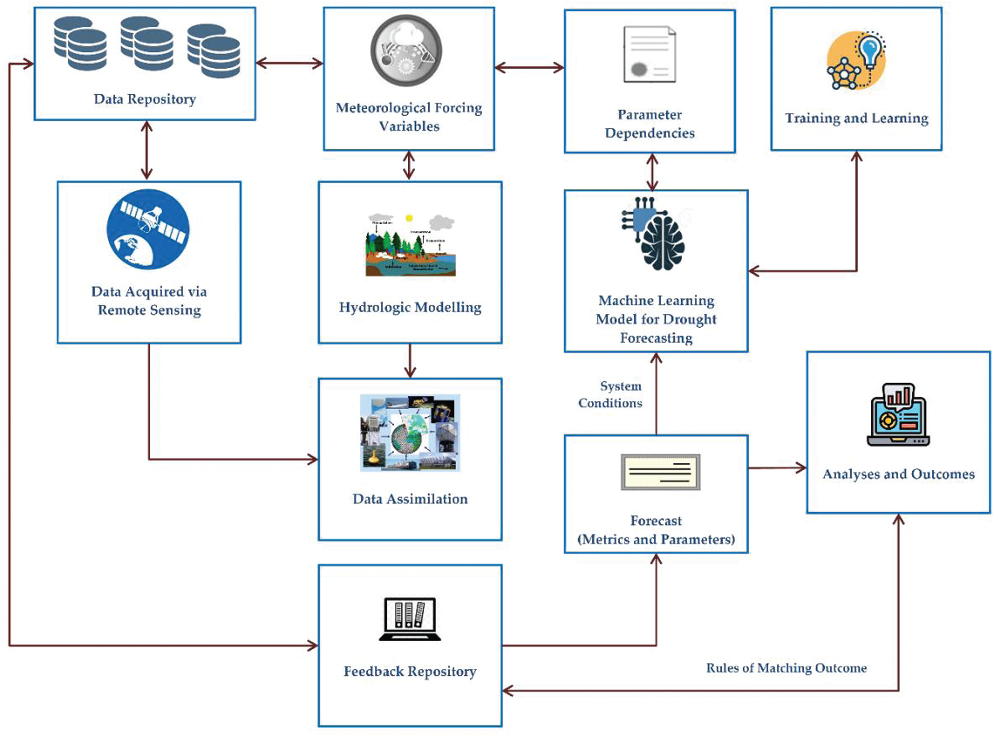
Figure 7: An archetypal portrayal of machine learning (ML)-based operational model for drought forecasting
Further, the model can be devised appropriately using multiple drought parameters and obtaining the prediction's efficiency with a hybrid classifier. For instance, four drought predictor values can be calculated. Based on the four parameters’ values, rules are created by the rule-based classifier, and drought severity can be predicted. The indices used for finding the drought severity are SPI, Aridity anomaly, PDSI, and NDVI. The record from 1950 can be used in predicting the values of the indices. The indices are considered as features for classification. Based on the output, the rule-based classifier unit sets the rules, and the output gets determined. Instead of using a single classifier, multiple rule-based classifiers can be used in prediction. So each classifier in the multiple classifiers units would give an output prediction. A fusion algorithm might be required to finalize the best from the multiple outputs. The fusion algorithms like the major voting or Dempster Shafer approach can predict the final output. The drought severity output can be measured in three levels Low, Moderate, and severe. Moreover, satellite or in-situ data shall also be incorporated for improving meteorological and hydrological drought forecasting.
Drought is a very complex natural hazard for forecasting and handling. It is well understood from the review that many factors influence the drought forecasting process. There are numerous drought indices, including climatic and oceanic factors, the forecast's leading time, pre-processing climatic data with a wavelet, and other transforms. Also, there are several ML techniques for drought forecasting. When comparing the direct and recursive models, it is seen that the direct models perform well at SPI's longer time scales and recursive models at shorter time scales. Shirmohammadi et al. [82] proved the exemplary performance of wavelet ANFIS methods with SPI. Prasad et al. [98] achieved the minimum RMSE value of 0.201 using ANN, and HMM [116] had the maximum RMSE of 0.852. Kaur et al. [156] got a maximum prediction accuracy of 95% with ANN-GA. The RMSE value for SPEI prediction done by Park et al. [124] using ANN was 0.338 and by Tian et al. [106] with SVM was 0.429. In Hosseini-Moghari et al. [90], R2 values of direct MLP, RBF, and GRNN are 0.627, 0.601, and 0.619; for recursive, the R2 values are 0.588, 0.563, and 0.598 a notable decrease with the recursive method was found. Bayesian model for PHDI got an RPS score of 1.744. The wavelet ANFIS and ensemble-ANFIS [157] are some of the superior models for drought forecasting. Machine learning models with Neural Networks give their best output in forecasting [158,159] and time series analysis [160]. The Deep learning methods success in other applications is proved well [161].
Drought is a natural hazard, extremely complex to forecast and handle. The paper critically reviews the drought indices like climatic and oceanic factors, the forecast's leading time, pre-processing climatic data with a wavelet, and other transforms and ML techniques for drought forecasting. Many factors influence the drought forecasting process. The direct models perform well at SPI's longer time scales and recursive models at shorter time scales. Many studies successfully used wavelet ANFIS. The paper also explains the fundamental concepts of the drought, its types, and its impact. This review paper can be a brilliant resource for researchers in drought forecasting and mitigation. It elaborates the drought indices, ML algorithms for drought forecasting, and the geographical area of their application in various studies.
As future work, a more comprehensive and extensive review of ML techniques for drought forecasting is proposed especially reviewing feature selection, feature extraction, and dimensionality reduction methods. A tool can also be developed for drought forecasting professionals to decide the most suitable approach based on the available data and accuracy. Furthermore, benchmark datasets can be made available as open-source to evaluate the performance of various ML techniques for drought forecasting.
Funding Statement: The authors received no specific funding for this study.
Conflicts of Interest: The authors declare that they have no conflicts of interest to report regarding the present study.
1. NDMC (2006a). What is drought? understanding and defining drought. National Climatic Data Center. http://www.drought.unl.edu/whatis/concept.htm. [Google Scholar]
2. Dracup, J. A., Lee, K. S., Paulson, E. G. (1980). On the definition of droughts. Water Resources Research, American Geophysical Union, 16(2), 297–302. DOI 10.1029/WR016i002p00297. [Google Scholar] [CrossRef]
3. Wilhite, D. A. (1990). The Enigma of Drought. Drought assessment, management, and planning: Theory and case studies, vol. 2, pp. 3–15. Boston: Kluwer Academic Publishers. [Google Scholar]
4. Victor, M. P. (1999). Hydrological drought. http://ponce.sdsu.edu/. [Google Scholar]
5. NDMC (2006b). Impacts of drought. National Climatic Data Center. http://www.drought.unl.edu/risk/impacts.htm. [Google Scholar]
6. Keetch, J. J., Byram, G. M. (1968). A drought index for forest fire control. United States Department of Agriculture Forest Service Research Paper SE-38, South Eastern Forest Experiment Station, Asheville. [Google Scholar]
7. Guttman, N. B. (1999). Accepting the standardized precipitation index: A calculation algorithm. Journal of the American Water Resources Association, 35(2), 311–322. DOI 10.1111/j.1752-1688.1999.tb03592.x. [Google Scholar] [CrossRef]
8. Guttman, N. B. (1998). Comparing the palmer drought index and the standardized precipitation index. Journal of the American Water Resources Association, 34(1), 113–121. DOI 10.1111/j.1752-1688.1998.tb05964.x. [Google Scholar] [CrossRef]
9. Svoboda, M., Fuchs, B. (2016). Handbook of drought indicators and indices. Lincoln, NE, USA: National Drought Mitigation Center. [Google Scholar]
10. Lyon, B. (2004). The strength of El niño and the spatial extent of tropical drought. Geophysical Research Letters, 31, L21204. DOI 10.1029/2004GL020901. [Google Scholar] [CrossRef]
11. Baltas, E. (2007). Spatial distribution of climatic indices in northern Greece. Meteorological Applications, 14, 69–78. DOI 10.1002/met.7. [Google Scholar] [CrossRef]
12. Wu, H., Hayes, M. J., Weiss, A., Hu, Q. (2001). An evaluation of the standardized precipitation index, the China-z index and the statistical Z-score. International Journal of Climatology, 21, 745–758. DOI 10.1002/joc.658. [Google Scholar] [CrossRef]
13. Palmer, W. C. (1968). Keeping track of crop moisture conditions nationwide: The crop moisture index. Weather Wise, 21, 156–161. DOI 10.1080/00431672.1968.9932814. [Google Scholar] [CrossRef]
14. Bhalme, H. N., Mooley, D. A. (1980). Large-scale droughts/floods and monsoon circulation. Monthly Weather Review, 108, 1197–1211. DOI 10.1175/1520-0493(1980)108<1197:LSDAMC>2.0.CO;2. [Google Scholar] [CrossRef]
15. Tsakiris, G., Vangelis, H. (2005). Establishing a drought index incorporating evapotranspiration. European Water, 10, 3–11. [Google Scholar]
16. Byun, H. R., Wilhite, D. A. (1996). Daily quantification of drought severity and duration. Journal of Climate, 5, 1181–1201. DOI 10.1175/1520-0442(1999)012<2747:OQODSA>2.0.CO;2. [Google Scholar] [CrossRef]
17. Alley, W. M. (1984). The palmer drought severity index: Limitations and assumptions. Journal of Applied Meteorology, 23, 1100–1109. DOI 10.1175/1520-0450(1984)023<1100:TPDSIL>2.0.CO;2. [Google Scholar] [CrossRef]
18. Kraus, E. B. (1977). Subtropical droughts and cross-equatorial energy transports. Monthly Weather Review, 8, 1009–1018. DOI 10.1175/1520-0493(1977)105<1009:SDACEE>2.0.CO;2. [Google Scholar] [CrossRef]
19. Wells, N., Goddard, S., Hayes, M. J. (2004). A self-calibrating palmer drought severity index. Journal of Climate, 17, 2335–2351. DOI 10.1175/1520-0442(2004)017%3c2335:ASPDSI%3e2.0.CO;2. [Google Scholar] [CrossRef]
20. Katz, R. W., Glantz, M. H. (1986). Anatomy of a rainfall index. Monthly Weather Review, 114, 764–771. DOI 10.1175/1520-0493(1986)114<0764:AOARI>2.0.CO;2. [Google Scholar] [CrossRef]
21. Vicente-Serrano, S. M., Begueria, S., Lopez-Moreno, J. I. (2010). A multi-scalar drought index sensitive to global warming: The standardized precipitation evapotranspiration index. Journal of Climate, 23, 1696–1718. DOI 10.1175/2009JCLI2909.1. [Google Scholar] [CrossRef]
22. Woli, P., Jones, J. W., Ingram, K. T., Fraisse, C. W. (2012). Agricultural reference index for drought (ARID). Agronomy Journal, 104, 287–300. DOI 10.2134/agronj2011.0286. [Google Scholar] [CrossRef]
23. Meyer, S. J., Hubbard, K. G., Wilhite, D. A. (1993). A crop-specific drought index for corn. I. Model Development and Validation. Agronomy Journal, 85, 388–395. DOI 10.2134/agronj1993.00021962008500020040x. [Google Scholar] [CrossRef]
24. Meyer, S. J., Hubbard, K. G., Wilhite, D. A. (1993). A crop-specific drought index for corn. II. Application in Drought Monitoring and Assessment. Agronomy Journal, 85, 396–399. DOI 10.2134/agronj1993.00021962008500020041x. [Google Scholar] [CrossRef]
25. Weghorst, K. (1996). The reclamation drought index: Guidelines and practical applications. Bureau of Reclamation, Denver, CO, USA. [Google Scholar]
26. Bergman, K. H., Sabol, P., Miskus, D. (1988). Experimental indices for monitoring global drought conditions. Proceedings of 13th Annual Climate Diagnostics Workshop, United States Department of Commerce, Cambridge, MA, USA. [Google Scholar]
27. Narasimhan, B., Srinivasan, R. (2005). Development and evaluation of soil moisture deficit index (SMDI) and evapotranspiration deficit index (ETDI) for agricultural drought monitoring. Agricultural and Forest Meteorology, 133, 69–88. DOI 10.1016/j.agrformet.2005.07.012. [Google Scholar] [CrossRef]
28. British Columbia Ministry of Agriculture (2015). Soil water storage capacity and available soil moisture. Water Conservation Fact Sheet. Abbotsford, British Columbia, Canada: Ministry of Agriculture. [Google Scholar]
29. Palmer, W. C. (1965). Meteorological drought. Research Paper No. 45. US Weather Bureau, Washington DC, USA. [Google Scholar]
30. Gusyev, M. A., Hasegawa, A., Magome, J., Kuribayashi, D., Sawano, H. et al. (2015). Drought assessment in the pampanga river basin, the Philippines. Part 1: A Role of dam Infrastructure in Historical Droughts. Proceedings of the 21st International Congress on Modelling and Simulation, Broadbeach, Queensland, Australia. [Google Scholar]
31. Telesca, L., Lovallo, M., Lopez-Moreno, I. (2012). Vicente-serrano. S. investigation of scaling properties in monthly streamflow and standardized streamflow index time series in the ebro basin (Spain). Physica A: Statistical Mechanics and its Applications, 391, 1662–1678. DOI 10.1016/j.physa.2011.10.023. [Google Scholar] [CrossRef]
32. Bhuiyan, C. (2004). Various drought indices for monitoring drought condition in aravalli terrain of India. Proceedings of the 20th ISPRS Conference. International Society for Photogrammetry and Remote Sensing, Istanbul, Turkey. [Google Scholar]
33. Nalbantis, I., Tsakiris, G. (2008). Assessment of hydrological drought revisited. Water Resources Management, 23, 881–897. DOI 10.1007/s11269-008-9305-1. [Google Scholar] [CrossRef]
34. Doesken, N. J., McKee, T. B., Kleist, J. (1991). Development of a surface water supply index for the western United States. Climatology Report, 91-3. Colorado Climate Center. [Google Scholar]
35. Keyantash, J. A., Dracup, J. A. (2004). An aggregate drought index: Assessing drought severity based on fluctuations in the hydrologic cycle and surface water storage. Water Resources Research, 40, W09304. DOI 10.1029/2003WR002610. [Google Scholar] [CrossRef]
36. Staudinger, M., Stahl, K., Seibert, J. (2014). A drought index accounting for snow. Water Resources Research, 50, 7861–7872. DOI 10.1002/2013WR015143. [Google Scholar] [CrossRef]
37. Huete, A., Didan, K., Miura, T., Rodriguez, E. P., Gao, X. et al. (2002). Overview of the radiometric and biophysical performance of the MODIS vegetation indices. Remote Sensing of Environment, 83, 195–213. DOI 10.1016/S0034-4257(02)00096-2. [Google Scholar] [CrossRef]
38. Anderson, M. C., Hain, C., Wardlow, B., Pimstein, A., Mecikalski, J. R. et al. (2011). Evaluation of drought indices based on thermal remote sensing of evapotranspiration over the continental United States. Journal of Climate, 24, 2025–2044. DOI 10.1175/2010JCLI3812.1. [Google Scholar] [CrossRef]
39. Kogan, F. N. (1995). Droughts of the late 1980s in the United States as derived from NOAA polar-orbiting satellite data. Bulletin of the American Meteorology Society, 76, 655–668. DOI 10.1175/1520-0477(1995)076<0655:DOTLIT.2.0.CO;2. [Google Scholar] [CrossRef]
40. Kogan, F. N. (1995). Application of vegetation index and brightness temperature for drought detection. Advances in Space Research, 15, 91–100. DOI 10.1016/0273-1177(95)00079-T. [Google Scholar] [CrossRef]
41. Liu, W. T., Kogan, F. N. (1996). Monitoring regional drought using the vegetation condition index. International Journal of Remote Sensing, 17, 2761–2782. DOI 10.1080/01431169608949106. [Google Scholar] [CrossRef]
42. Brown, J. F., Wardlow, B. D., Tadesse, T., Hayes, M. J., Reed, B. C. (2008). The vegetation drought response index (VegDRIA new integrated approach for monitoring drought stress in vegetation. GISCience & Remote Sensing, 45, 16–46. DOI 10.2747/1548-1603.45.1.16. [Google Scholar] [CrossRef]
43. Kogan, F. N. (1990). Remote sensing of weather impacts on vegetation in non-homogeneous areas. International Journal of Remote Sensing, 11, 1405–1419. DOI 10.1080/01431169008955102. [Google Scholar] [CrossRef]
44. Verdin, J., Klaver, R. (2002). Grid-cell-based crop water accounting for the famine early warning system. Hydrological Processes, 16, 1617–1630. DOI 10.1002/(ISSN)1099-1085. [Google Scholar] [CrossRef]
45. Chandrasekar, K., Sesha Sai, M. V. R., Roy, P. S., Dwevedi, R. S. (2010). Land surface water index (LSWI) response to rainfall and NDVI using the MODIS vegetation index product. International Journal of Remote Sensing, 31, 3987–4005. DOI 10.1080/01431160802575653. [Google Scholar] [CrossRef]
46. Gao, B. C. (1996). NDWI—A normalized difference water index for remote sensing of vegetation liquid water from space. Remote Sensing of Environment, 58, 257–266. DOI 10.1016/S0034-4257(96)00067-3. [Google Scholar] [CrossRef]
47. Huete, A. R. (1998). A soil-adjusted vegetation index (SAVI). Remote Sensing of Environment, 25, 295–309. DOI 10.1016/0034-4257(88)90106-X. [Google Scholar] [CrossRef]
48. NCEI (2021). Southern Oscillation Index (SOI). https://www.ncdc.noaa.gov/teleconnections/enso/indicators/soi/. [Google Scholar]
49. Mishra, D., Goswami, S., Matin, S., Sarup, J. (2021). Analyzing the extent of drought in the rajasthan state of India using vegetation condition index and standardized precipitation index. Modeling Earth Systems and Environment, 1–10. DOI 10.1007/s40808-021-01102-x. [Google Scholar] [CrossRef]
50. Wei, W., Zhang, J., Zhou, L., Xie, B., Zhou, J. et al. (2021). Comparative evaluation of drought indices for monitoring drought based on remote sensing data. Environmental Science and Pollution Research, 28(16), 20408–20425. DOI 10.1007/s11356-020-12120-0. [Google Scholar] [CrossRef]
51. Bai, X. J., Kang, H. X., Wang, P. X., Liu, Z. (2021). Effectiveness of upscaling the vegetation temperature condition index retrieved from landsat data using an algorithm combining the trend surface analysis and the spatial variation weight method. European Journal of Remote Sensing, 54(1), 29–41. DOI 10.1080/22797254.2020.1847603. [Google Scholar] [CrossRef]
52. Kirkham, M. B. (2014). Potential evapotranspiration. Principles of soil and plant water relations (Second Edition), pp. 501–514. DOI 10.1016/B978-0-12-420022-7.00028-8. [Google Scholar] [CrossRef]
53. Homdee, T., Pongput, K., Kanae, S. (2016). A comparative performance analysis of three standardized climatic drought indices in the Chi River basin, Thailand. Agriculture and Natural Resources, 50(3), 211–219. DOI 10.1016/j.anres.2016.02.002. [Google Scholar] [CrossRef]
54. Zhu, N., Xu, J., Li, W., Li, K., Zhou, C. (2018). A comprehensive approach to assess the hydrological drought of inland river basin in northwest China. Atmosphere, 9, 370. DOI 10.3390/atmos9100370. [Google Scholar] [CrossRef]
55. Greve, P., Roderick, M. L., Ukkola, A. M., Wada, Y. (2019). The aridity index under global warming. Environmental Research Letters, 14(12), 124006. DOI 10.1088/1748-9326/ab5046. [Google Scholar] [CrossRef]
56. Dobri, R. V., Sfîcă, L., Amihăesei, V. A., Apostol, L., Țîmpu, S. (2021). Drought extent and severity on arable lands in Romania derived from normalized difference drought index (2001–2020). Remote Sensing, 13(8), 1478. DOI 10.3390/rs13081478. [Google Scholar] [CrossRef]
57. Burke, E. J. (2011). Understanding the sensitivity of different drought metrics to the drivers of drought under increased atmospheric CO2. Journal of Hydrometeorology, 12(6), 1378–1394. DOI 10.1175/2011JHM1386.1. [Google Scholar] [CrossRef]
58. Bos, M. G., Kselik, R. A. L., Allen, R. G., Molden, D. J. (2009). Water requirements for irrigation and the environment, vol. 3, pp. 81–102. Springer Science and Business Media: Dordrecht, The Netherlands. DOI 10.1007/978-1-4020-8948-0. [Google Scholar] [CrossRef]
59. Elavarasan, D., Vincent, D. R., Sharma, V., Zomaya, A. Y., Srinivasan, K. (2018). Forecasting yield by integrating agrarian factors and machine learning models: A survey. Computers and Electronics in Agriculture, 155, 257–282. DOI 10.1016/j.compag.2018.10.024. [Google Scholar] [CrossRef]
60. Moriasi, D. N., Arnold, J. G., van Liew, M. W., Bingner, R. L., Harmel, R. D. et al. (2007). Model evaluation guidelines for systematic quantification of accuracy in watershed simulations. Transactions of the ASABE, 50(3), 885–900. DOI 10.13031/2013.23153. [Google Scholar] [CrossRef]
61. Srinivasan, K., Garg, L., Datta, D., Alaboudi, A. A., Jhanjhi, N. Z. et al. (2021). Performance comparison of deep CNN models for detecting driver's distraction. Computers, Materials & Continua (in Press). [Google Scholar]
62. Jayalakshmi, M., Garg, L., Maharajan, K., Jayakumar, K., Srinivasan, K. (2021). Fuzzy logic-based health monitoring system for COVID'19 patients. Computers, Materials & Continua, 67(2), 2431–2447. DOI 10.32604/cmc.2021.015352. [Google Scholar] [CrossRef]
63. Garg, R., Brennan, L., Price, R. K., Wallace, J., Strain, J. J. (2016). Using NMR-based metabolomics to evaluate postprandial urinary responses following consumption of minimally processed wheat bran or wheat aleurone by men and women. Nutrients, 8(2), 96. DOI 10.3390/nu8020096. [Google Scholar] [CrossRef]
64. Garg, L., Dauwels, J., Earnest, A., Pang, L. (2014). Tensor-based methods for handling missing data in quality-of life questionnaires. IEEE Journal of Biomedical and Health Informatics, 18(5), 1571–1580. DOI 10.1109/JBHI.2013.2288803. [Google Scholar] [CrossRef]
65. Garg, L., McClean, S. I., Barton, M. (2014). Can management science methods do more to improve healthcare? International Journal of Inventions in Research, Engineering Science and Technology, 8, 8–18. [Google Scholar]
66. Garg, L., McClean, S. I., Meenan, B. J., Millard, P. H. (2011). Phase-type survival trees and mixed distribution survival trees for clustering patients’ hospital length of stay. Informatica, 22(1), 57–72. DOI 10.15388/Informatica.2011.314. [Google Scholar] [CrossRef]
67. Garg, L., McClean, S. I., Barton, M., Meenan, B. J., Fullerton, K. (2010). The extended mixture distribution survival tree-based analysis for clustering and patient pathway prognostication in a stroke care unit. International Journal of Information Sciences and Application, 2(4), 671–675. DOI 10.1080/03610926.2012.725262. [Google Scholar] [CrossRef]
68. McClean, S., Barton, M., Garg, L., Fullerton, K. (2011). Modeling framework that combines markov models and discrete-event simulation for stroke patient care. ACM Transactions on Modeling and Computer Simulation (TOMACS), 21(4), 1–26. DOI 10.1145/2000494.2000498. [Google Scholar] [CrossRef]
69. Papadapoulou, A., Tsaklidis, G., McClean, S. I., Garg, L. (2011). On the moments and the distribution of the cost of a semi markov model for healthcare systems. Methodology and Computing in Applied Probability, 4(3), 717–737. DOI 10.1007/s11009-011-9260-9. [Google Scholar] [CrossRef]
70. Garg, G., Prasad, G., Garg, L., Coyle, D. (2011). Gaussian mixture models for brain activation detection from fMRI data. International Journal of Bioelectromagnetism, 13(4), 255–260. [Google Scholar]
71. Garg, L., McClean, S. I., Meenan, B. J., Millard, P. H. (2010). A non-homogeneous discrete-time markov model for admission scheduling and resource planning in a cost or capacity constrained healthcare system. Health Care Management Science, 13(2), 155–169. DOI 10.1007/s10729-009-9120-0. [Google Scholar] [CrossRef]
72. Garg, L., McClean, S. I., Meenan, B. J., Millard, P. H. (2009). Non-homogeneous markov models for sequential pattern mining of healthcare data. IMA Journal of Management Mathematics, 20(4), 327–344. DOI 10.1093/imaman/dpn030. [Google Scholar] [CrossRef]
73. Bugeja, S., Garg, L., Audu, E. E. (2016). A novel method of EEG data acquisition, feature extraction and feature space creation for early detection of epileptic seizures. 38th Annual International Conference of the IEEE Engineering in Medicine and Biology Society (EMBC-2016). Orlando, Florida, USA. DOI 10.1109/EMBC.2016.7590831. [Google Scholar] [CrossRef]
74. Bacanli, U. G., Firat, M., Dikbas, F. (2009). Adaptive neuro-fuzzy inference system for drought forecasting. Stochastic Environmental Research and Risk Assessment, 23, 1143–1154. DOI 10.1007/s00477-008-0288-5. [Google Scholar] [CrossRef]
75. Cutore, P., Mauro, G., Cancelliere, A. (2009). Forecasting palmer index using neural networks. Journal of Hydrologic Engineering, 14, 588–595. DOI 10.1061/(ASCE)HE.1943-5584.0000028. [Google Scholar] [CrossRef]
76. Dastorani, M. T., Afkhami, H., Shariffdarani, H., Dastorani, M. (2010). Application of ANN and ANFIS models on dryland precipitation prediction case study: Yazd in central Iran. Journal of Applied Sciences, 10(20), 2387–2394. DOI 10.3923/jas.2010.2387.2394. [Google Scholar] [CrossRef]
77. Marj, A. F., Meijerink, A. M. J. (2011). Agricultural drought forecasting using satellite images, climate indices and artificial neural network. International Journal of Remote Sensing, 32, 9707–9719. DOI 10.1080/01431161.2011.575896. [Google Scholar] [CrossRef]
78. Barua, S., Ng, A. W. M., Perera, B. J. C. (2012). Artificial neural network-based drought forecasting using a nonlinear aggregated drought index. Journal of Hydrologic Engineering, 17, 1408–1413. DOI 10.1061/ASCEHE.1943-5584.0000574. [Google Scholar] [CrossRef]
79. Belayneh, A., Adamowski, J., Khalil, B., Ozga-Zielinski, B. (2013). Long-term SPI drought forecasting in the awash river basin in Ethiopia using wavelet neural networks and wavelet support vector regression models. Journal of Hydrology, 508, 418–429. DOI 10.1016/j.jhydrol.2013.10.052. [Google Scholar] [CrossRef]
80. Woli, P., Jones, J., Ingram, K., Paz, J. (2013). Forecasting drought using the agricultural reference index for drought ARID: A case study. Weather Forecast, 28, 427–443. DOI 10.1175/WAF-D-12-00036.1. [Google Scholar] [CrossRef]
81. Belayneh, A., Adamowski, J., Khalil, B., Quilty, J. (2016). Coupling machine learning methods with wavelet transforms and the bootstrap and boosting ensemble approaches for drought prediction. Atmospheric Research, 172, 37–47. DOI 10.1016/j.atmosres.2015.12.017. [Google Scholar] [CrossRef]
82. Shirmohammadi, B., Moradi, H., Moosavi, V., Semiromi, M. T., Zeinali, A. (2013). Fore-casting of meteorological drought using wavelet-aNFIS hybrid model for different time steps case study: Southeastern part of east Azerbaijan province Iran. Natural Hazards, 69, 389–402. DOI 10.1007/s11069-013-0716-9. [Google Scholar] [CrossRef]
83. Masinde, M. (2014). Artificial neural networks models for predicting effective drought index: Factoring effects of rainfall variability. Mitigation and Adaptation Strategies for Global Change, 19, 1139–1162. DOI 10.1007/s11027-013-9464-0. [Google Scholar] [CrossRef]
84. Wambua, R. M., Mutua, B. M., Raude, J. M. (2014). Drought forecasting using indices and artificial neural networks for upper Tana River Basin, Kenya–A review concept. Journal of Civil & Environmental Engineering, 4(4), 152. DOI 10.4172/2165-784X.1000152. [Google Scholar] [CrossRef]
85. Jalalkamali, A., Moradi, M., Moradi, N. (2015). Application of several artificial intelligence models and ARIMAX model for forecasting drought using the standardized precipitation index. International Journal of Environmental Science and Technology, 12, 1201–1210. DOI 10.1007/s13762-014-0717-6. [Google Scholar] [CrossRef]
86. Belayneh, A., Adamowski, J. (2012). Standard precipitation index drought forecasting using neural networks, wavelet neural networks, and support vector regression. Applied computational intelligence and soft computing, vol. 2012, pp. 1–13. DOI 10.1155/2012/794061. [Google Scholar] [CrossRef]
87. Deo, R. C., Şahin, M. (2015). Application of the artificial neural network model for prediction of monthly standardized precipitation and evapotranspiration index using hydrometeorological parameters and climate indices in Eastern Australia. Atmospheric Research, 161, 65–81. DOI 10.1016/j.atmosres.2015.03.018. [Google Scholar] [CrossRef]
88. Maca, P., Pech, P. (2016). Forecasting SPEI and SPI drought indices using the integrated artificial neural networks. Computational intelligence and neuroscience, vol. 2016, pp. 1–17. DOI 10.1155/2016/3868519. [Google Scholar] [CrossRef]
89. Kousari, M. R., Hosseini, M. E., Ahani, H., Hakimelahi, H. (2017). Introducing an operational method to forecast long-term regional drought based on the application of artificial intelligence capabilities. Theoretical and Applied Climatology, 127(1–2), 361–380. DOI 10.1007/s00704-015-1624-6. [Google Scholar] [CrossRef]
90. Hosseini-Moghari, S. M., Araghinejad, S. (2015). Monthly and seasonal drought forecasting using statistical neural networks. Environmental Earth Sciences, 74(1), 397–412. DOI 10.1007/s12665-015-4047-x. [Google Scholar] [CrossRef]
91. Deo, R. C., Tiwari, M. K., Adamowski, J. F., Quilty, J. M. (2016). Forecasting effective drought index using a wavelet extreme learning machine (W-eLM) model. Stochastic Environmental Research and Risk Assessment, 31(5), 1211–1240. DOI 10.1007/s00477-016-1265-z. [Google Scholar] [CrossRef]
92. Rezaeianzadeh, M., Stein, A., Cox, J. P. (2016). Drought forecasting using markov chain model and artificial neural networks. Water Resources Management, 30(7), 2245–2259. DOI 10.1007/s11269-016-1283-0. [Google Scholar] [CrossRef]
93. Borji, M., Malekian, A., Salajegheh, A., Ghadimi, M. (2016). Multi-time-scale analysis of hydrological drought forecasting using support vector regression (SVR) and artificial neural networks (ANN). Arabian Journal of Geosciences, 9(19), 1–10. DOI 10.1007/s12517-016-2750-x. [Google Scholar] [CrossRef]
94. Djerbouai, S., Souag-Gamane, D. (2016). Drought forecasting using neural networks, wavelet neural networks, and stochastic models: Case of the algerois basin in north Algeria. Water Resources Management, 30(7), 2445–2464. DOI 10.1007/s11269-016-1298-6. [Google Scholar] [CrossRef]
95. Le, M. H., Perez, G. C., Solomatine, D., Nguyen, L. B. (2016). Meteorological drought forecasting based on climate signals using artificial neural network–A case study in khanhhoa province Vietnam. Procedia Engineering, 154, 1169–1175. DOI 10.1016/j.proeng.2016.07.528. [Google Scholar] [CrossRef]
96. Ibrahimi, A., Baali, A. (2018). Application of several artificial intelligence models for forecasting meteorological drought using the standardized precipitation index in the saiss plain (Northern Morocco). International Journal of Intelligent Engineering and Systems, 11(1), 267–275. DOI 10.22266/ijies. [Google Scholar] [CrossRef]
97. Ali, Z., Hussain, I., Faisal, M., Nazir, H. M., Hussain, T. et al. (2017). Forecasting drought using multilayer perceptron artificial neural network model. Advances in meteorology, vol. 2017, pp. 1–9. DOI 10.1155/2017/5681308. [Google Scholar] [CrossRef]
98. Prasad, R. D., Ravinesh, C., Li, Y., Maraseni, T. (2017). Input selection and performance optimization of ANN-based streamflow forecasts in the drought-prone Murray darling basin region using IIS and MODWT algorithm. Atmospheric Research, 197, 42–63. DOI 10.1016/j.atmosres.2017.06.014. [Google Scholar] [CrossRef]
99. Adeyemi, O., Grove, I., Peets, S., Domun, Y., Norton, T. (2018). Dynamic neural network modelling of soil moisture content for predictive irrigation scheduling. Sensors, 18(10), 3408. DOI 10.3390/s18103408. [Google Scholar] [CrossRef]
100. Zhang, R., Chen, Z. Y., Xu, L. J., Ou, C. Q. (2019). Meteorological drought forecasting based on a statistical model with machine learning techniques in Shaanxi Province, China. Science of the Total Environment, 665, 338–346. DOI 10.1016/j.scitotenv.2019.01.431.
101. Deng, J., Chen, X., Du, Z., Zhang, Y. (2011). Soil water simulation and prediction using stochastic models based on LS-sVM for Red soil region of China. Water Resources Management, 25(11), 2823–2836. DOI 10.1007/s11269-011-9840-z.
102. Kisi, O., Cimen, M. (2011). A wavelet-support vector machine conjunction model for monthly streamflow forecasting. Journal of Hydrology, 399(1–2), 132–140. DOI 10.1016/j.jhydrol.2010.12.041.
103. Chiang, J. L., Tsai, Y. S. (2013). Reservoir drought prediction using two-stage SVM. Applied Mechanics and Materials, 284, 1473–1477. DOI 10.4028/www.scientific.net/AMM.284-287.1473.
104. Ganguli, P., Reddy, M. J. (2014). Ensemble prediction of regional droughts using climate inputs and SVM-copula approach. Hydrol Process, 28(19), 4989–5009. DOI 10.1002/hyp.9966.
105. Chiang, J. L., Tsai, Y. S. (2012). Reservoir drought prediction using support vector machines. Applied Mechanics and Materials, 145, 455–459. Switzerland: Trans Tech Publications, Ltd. DOI 10.4028/www.scientific.net/AMM.145.455.
106. Tian, Y., Xu, Y. P., Wang, G. (2018). Agricultural drought prediction using climate indices based on support vector regression in Xiangjiang River Basin. Science of the Total Environment, 622, 710–720. DOI 10.1016/j.scitotenv.2017.12.025.
107. Keskin, M. E., Terzi, Ö., Taylan, E. D., Küçükyaman, D. (2009). Meteorological drought analysis using data-driven models for the lakes district, Turkey. Hydrological Sciences Journal, 54, 1114–1124. DOI 10.1623/hysj.54.6.1114.
108. Ozger, M., Mishra, A. K., Singh, V. P. (2011). Estimating palmer drought severity index using a wavelet fuzzy logic model based on meteorological variables. International Journal of Climatology, 31(13), 2021–2032. DOI 10.1002/joc.2215.
109. Mehr, A. D., Kahya, E., Ozger, M. (2014). A gene-wavelet model for long lead time drought forecasting. Journal of Hydrology, 517, 691–699. DOI 10.1016/j.jhydrol.2014.06.012.
110. Madadgar, S., Moradkhani, H. (2014). Spatio-temporal drought forecasting within Bayesian networks. Journal of Hydrology, 512, 134–146. DOI 10.1016/j.jhydrol.2014.02.039.
111. Bae, D. H., Son, K. H., So, J. M. (2017). Utilization of the Bayesian method to improve hydrological drought prediction accuracy. Water Resources Management, 31(11), 3527–3541. DOI 10.1007/s11269-017-1682-x.
112. Sattar, M. N., Kim, T. W. (2018). Probabilistic characteristics of lag time between meteorological and hydrological droughts using a Bayesian model. Terrestrial, Atmospheric & Oceanic Sciences, 29(6), 1–12. DOI 10.3319/TAO.2018.07.01.01.
113. Chen, S., Muhammad, W., Lee, J. H., Kim, T. W. (2018). Assessment of probabilistic multi-index drought using a dynamic naive Bayesian classifier. Water Resources Management, 32(13), 4359–4374. DOI 10.1007/s11269-018-2062-x.
114. Shin, J. Y., Ajmal, M., Yoo, J., Kim, T. W. (2016). A Bayesian network-based probabilistic framework for drought forecasting and outlook. Advances in Meteorology, 1–10. DOI 10.1155/2016/9472605.
115. Shin, J. Y., Kwon, H. H., Lee, J. H., Kim, T. W. (2020). Probabilistic long-term hydrological drought forecast using Bayesian networks and drought propagation. Meteorological Applications, 27(1), e1827. DOI 10.1002/met.1827.
116. Chen, J., Yang, Y. (2012). SPI-Based regional drought prediction using weighted markov chain model. Research Journal of Applied Sciences, Engineering and Technology, 421, 4293–4298.
117. Park, S., Im, J., Jang, E., Rhee, J. (2016). Drought assessment and monitoring through blending of multi-sensor indices using machine learning approaches for different climate regions. Agricultural and Forest Meteorology, 216, 157–169. DOI 10.1016/j.agrformet.2015.10.011.
118. Park, H., Kim, K., Lee, D. K. (2019). Prediction of severe drought area based on random forest: Using satellite image and topography data. Water, 11(4), 705. DOI 10.3390/w11040705.
119. Rahmat, S. N., Jayasuriya, N., Bhuiyan, M. A. (2016). Short-term droughts forecast using markov chain model in Victoria, Australia. Theoretical and Applied Climatology, 129(1), 445–457. DOI 10.1007/s00704-016-1785-y.
120. Chen, S., Shin, J. Y., Kim, T. W. (2016). Probabilistic forecasting of drought: A hidden markov model aggregated with the RCP 8.5 precipitation projection. Stochastic Environmental Research and Risk Assessment, 31(5), 1061–1076. DOI 10.1007/s00477-016-1279-6.
121. Khadr, M. (2016). Forecasting of meteorological drought using hidden markov model case study: The upper blue Nile River Basin Ethiopia. Ain Shams Engineering Journal, 7(1), 47–56. DOI 10.1016/j.asej.2015.11.005.
122. Nnaji, G. A., Clark, C. J., Chan-Hilton, A. B., Huang, W. (2016). Drought prediction in Apalachicola-Chattahoochee Flint River Basin using a semi-Markov model. Natural Hazards, 821(1), 267–297. DOI 10.1007/s11069-016-2201-8.
123. Shamshirband, S., Hashemi, S., Salimi, H., Samadianfard, S., Asadi, E. (2020). Predicting standardized streamflow index for hydrological drought using machine learning models. Engineering Applications of Computational Fluid Mechanics, 14(1), 339–350. DOI 10.1080/19942060.2020.1715844.
124. Park, S., Im, J., Han, D., Rhee, J. (2020). Short-term forecasting of satellite-based drought indices using their temporal patterns and numerical model output. Remote Sensing, 12(21), 3499. DOI 10.3390/rs12213499.
125. Mathivha, F., Sigauke, C., Chikoore, H., Odiyo, J. (2020). Short-term and medium-term drought forecasting using generalized additive models. Sustainability, 12, 4006. DOI 10.3390/su12104006.
126. Nabipour, N., Dehghani, M., Mosavi, A., Shamshirband, S. (2020). Short-term hydrological drought forecasting based on different nature-inspired optimization algorithms hybridized with artificial neural networks. IEEE Access, 8, 15210–15222. DOI 10.1109/Access.6287639.
127. Dikshit, A., Pradhan, B., Alamri, A. M. (2020). Short-term spatio-temporal drought forecasting using random forests model at New South Wales, Australia. Applied Sciences, 10(12), 4254. DOI 10.3390/app10124254.
128. Fung, K. F., Huang, Y. F., Koo, C. H., Mirzaei, M. (2020). Improved SVR machine learning models for agricultural drought prediction at downstream of Langat River Basin, Malaysia. Journal of Water and Climate Change, 11(4), 1383–1398. DOI 10.2166/wcc.2019.295.
129. Mokhtari, R., Akhoondzadeh, M. (2021). Data fusion and machine learning algorithms for drought forecasting using satellite data. Journal of the Earth and Space Physics, 46(4), 231–246. DOI 10.22059/jesphys.2020.299445.1007199.
130. Kisi, O., Gorgij, A. D., Zounemat-Kermani, M., Mahdavi-Meymand, A., Kim, S. (2019). Drought forecasting using novel heuristic methods in a semi-arid environment. Journal of Hydrology, 578, 1–11. DOI 10.1016/j.jhydrol.2019.124053.
131. Mulualem, G. M., Liou, Y. A. (2020). Application of artificial neural networks in forecasting a standardized precipitation evapotranspiration index for the Upper Blue Nile Basin. Water, 12(3), 643. DOI 10.3390/w12030643.
132. Moazenzadeh, R., Mohammadi, B., Shamshirband, S., Chau, K. W. (2018). Coupling a firefly algorithm with support vector regression to predict evaporation in northern Iran. Engineering Applications of Computational Fluid Mechanics, 12(1), 584–597. DOI 10.1080/19942060.2018.1482476.
133. Nalbantis, I. (2008). Evaluation of a hydrological drought index. European Water, 23(24), 67–77.
134. Alsumaiei, A. A., Alrashidi, M. S. (2020). Hydrometeorological drought forecasting in hyper-arid climates using nonlinear autoregressive neural networks. Water, 12, 2611. DOI 10.3390/w12092611.
135. Memarian, H., Bilondi, M. P., Rezaei, M. (2016). Drought prediction using co-active neuro-fuzzy inference system, validation, and uncertainty analysis case study: Birjand, Iran. Theoretical and Applied Climatology, 125, 541–554. DOI 10.1007/s00704-015-1532-9.
136. Tufaner, F., Qzbeyaz, A. (2020). Estimation and easy calculation of the palmer drought severity index from the meteorological data by using the advanced machine learning algorithms.Environmental Monitoring and Assessment, 192(9), 1–14. DOI 10.1007/s10661-020-08539-0.
137. Agboola, A. H., Gabriel, A. J., Aliyu, E. O., Alese, B. K. (2013). Development of a fuzzy logic based rainfall prediction model. International Journal of Engineering and Technology, 3(4), 427–435.
138. Mehr, A. D., Tur, R., Çalışkan, C., Tas, E. (2020). A novel fuzzy random forest model for meteorological drought classification and prediction in ungauged catchments. Pure and Applied Geophysics, 177(12), 5993–6006. DOI 10.1007/s00024-020-02609-7.
139. Avilés, A., Célleri, R., Paredes, J., Solera, A. (2015). Evaluation of markov chain based drought forecasts in an Andean regulated river basin using the skill scores RPS and GMSS. Water Resources Management, 29, 1949–1963. DOI 10.1007/s11269-015-0921-2.
140. Zhu, S., Luo, X. G., Chen, S., Xu, Z. Y. (2020). Improved hidden markov model incorporated with copula for probabilistic seasonal drought forecasting. Journal of Hydrologic Engineering, 25(6), 04020019. DOI 10.1061/(ASCE)HE.1943-5584.0001901.
141. Agana, N. A., Homaifar, A. (2018). EMD-Based predictive deep belief network for time series prediction: An application to drought forecasting. Hydrology, 5(18), 18. DOI 10.3390/hydrology5010018.
142. Chen, J., Jin, Q., Chao, J. (2012). Design of deep belief networks for short-term prediction of drought index using data in the huaihe river basin. Mathematical Problems in Engineering, 2012, 1–16. DOI 10.1155/2012/235929.
143. Poornima, S., Pushpalatha, M. (2019). Drought prediction based on SPI and SPEI with varying timescales using LSTM recurrent neural network. Soft Computing, 23, 1–14. DOI 10.1007/s00500-019-04120-1.
144. Zhu, S., Xu, Z., Luo, X., Liu, X., Wang, R. et al. (2021). Internal and external coupling of Gaussian mixture model and deep recurrent network for probabilistic drought forecasting. International Journal of Environmental Science and Technology, 18(5), 1221–1236. DOI 10.1007/s13762-020-02862-2.
145. Ali, M., Deo, R. C., Downs, N. J., Maraseni, T. (2018). Multi-stage committee based extreme learning machine model incorporating the influence of climate parameters and seasonality on drought forecasting. Computers and Electronics in Agriculture, 152, 149–165. DOI 10.1016/j.compag.2018.07.013.
146. Ali, M., Deo, R. C., Maraseni, T., Downs, N. J. (2019). Improving SPI-derived drought forecasts incorporating synoptic-scale climate indices in multi-phase multivariate empirical mode decomposition model hybridized with simulated. Journal of Hydrology, 576, 164–184. DOI 10.1016/j.jhydrol.2019.06.032.
147. Dikshit, A., Pradhan, B., Alamri, A. M. (2020). Temporal hydrological drought index forecasting for New South Wales, Australia using machine learning approaches. Atmosphere, 11, 585. DOI 10.3390/atmos11060585.
148. Han, J., Singh, V. P. (2020). Forecasting of droughts and tree mortality under global warming: A review of causative mechanisms and modeling methods. Journal of Water and Climate Change, 11(3), 600–632. DOI 10.2166/wcc.2020.239.
149. Bojang, P. O., Yang, T. C., Pham, Q. B., Yu, P. S. (2020). Linking singular spectrum analysis and machine learning for monthly rainfall forecasting. Applied Sciences, 10(9), 3224. DOI 10.3390/app10093224.
150. Kaur, A., Sood, S. K. (2019). Cloud-Fog based framework for drought prediction and forecasting using artificial neural network and genetic algorithm. Journal of Experimental & Theoretical Artificial Intelligence, 32, 273–289 DOI 10.1080/0952813x.2019.1647563.
151. Farokhnia, A., Morid, S., Byun, H. R. (2010). Application of global SST and SLP data for drought forecasting on Tehran plain using data mining and ANFIS techniques. Theoretical and Applied Climatology, 104(1), 71–81. DOI 10.1007/s00704-010-0317-4.
152. Khan, M. M. H., Muhammad, N. S., El-Shafie, A. (2020). Wavelet based hybrid ANN-aRIMA models for meteorological drought forecasting. Journal of Hydrology, 590, 125380. DOI 10.1016/j.jhydrol.2020.125380.
153. Malik, A., Kumar, A. (2020). Meteorological drought prediction using heuristic approaches based on effective drought index: A case study in uttarakhand. Arabian Journal of Geosciences, 13(6), 276. DOI 10.1007/s12517-020-5239-6.
154. Mohamadi, S., Sammen, S. S., Panahi, F., Ehteram, M., Kisi, O. et al. (2020). Zoning map for drought prediction using integrated machine learning models with a nomadic people optimization algorithm. Natural Hazards, 104(1), 537–579. DOI 10.1007/s11069-020-04180-9.
155. So, J. M., Lee, J. H., Bae, D. H. (2020). Development of a hydrological drought forecasting model using weather forecasting data from Glosea5. Water, 12, 2785. DOI 10.3390/w12102785.
156. Kaur, A., Sood, S. K. (2019). Artificial intelligence-based model for drought prediction and forecasting. The Computer Journal, 63(11), 1704–1712. DOI 10.1093/comjnl/bxz105.
157. Ali, M., Deo, R. C., Downs, N. J., Maraseni, T. (2018). An ensemble-aNFIS based uncertainty assessment model for forecasting multi-scalar standardized precipitation index. Atmospheric Research, 207, 155–180. DOI 10.1016/j.atmosres.2018.02.024.
158. Mohan, S., John, A., Abugabah, A., Adimoolam, M., Singh, S. K. et al. (2021). An approach to forecast impact of COVID-19 using supervised machine learning model. Software: Practice and Experience, Wiley.
159. Morgan, G., Srivastava, G., Muthu, B. A., Baskar, S., Shakeel, P. M. (2021). A response-aware traffic offloading scheme using regression machine learning for user-centric large scale internet of things. IEEE Internet of Things Journal, 8(5), 3360–3368. DOI 10.1109/JIoT.6488907.
160. Jha, S., Yang, E., Almagrabi, A. O., Bashir, A. K., Joshi, G. P. (2020). Comparative analysis of time series model and machine testing systems for crime forecasting. Neural Computing and Applications, 1–16. DOI 10.1007/s00521-020-04998-1.
161. Reddy, T., Bhattacharya, S., Maddikunta, P. K. R., Hakak, S., Khan, W. Z. et al. (2020). Antlion Re-sampling based deep neural network model for classification of imbalanced multimodal stroke dataset. Multimedia Tools and Applications, 1–25. DOI 10.1007/s11042-020-09988-y.
 | This work is licensed under a Creative Commons Attribution 4.0 International License, which permits unrestricted use, distribution, and reproduction in any medium, provided the original work is properly cited. |