| Computer Modeling in Engineering & Sciences |
DOI: 10.32604/cmes.2021.015183
ARTICLE
Stability Reliability of the Lateral Vibration of Footbridges Based on the IEVIE-SA Method
School of Civil Engineering and Transportation, South China University of Technology, Guangzhou, 510640, China
*Corresponding Author: Xiaolin Yu. Email: xlyu1@scut.edu.cn
Received: 29 November 2020; Accepted: 19 April 2021
Abstract: Research on the lateral vibrational stability of footbridges has attracted increasing attention in recent years. However, this stability contains a series of complex mechanisms, such as nonlinear vibration, random excitation, and random stability. The Lyapunov method is regarded as an effective tool for analyzing random vibrational stability; however, it is a qualitative method and can only provide a binary judgment for stability. This study proposes a new method, IEVIE–SA, which combines the energy method based on the comparison between the input energy and the variation of intrinsic energy (IEVIE) and the stochastic averaging (SA) method. The improved Nakamura model was used to describe the lateral nonlinear stochastic vibration of a footbridge, whereby the IEVIE method was used to establish the criteria for judging the lateral vibrational stability. Additionally, the SA method was used to deduce the corresponding backward Kolmogorov equation. Subsequently, the backward Kolmogorov equation was combined with the stability criterion established by the IEVIE method to analyze the first passage stability. The proposed method is a semi-analytical, quantitative method that only requires a small calculation. By applying the proposed method to the Millennium Bridge, method effectiveness was verified by comparing it with the Monte Carlo and traditional Lyapunov methods.
Keywords: Footbridge; vibration; stability; energy; stochastic; reliability
Research on footbridge vibrations consists of two primary directions: vertical and lateral. During vertical vibration, it is generally believed that pedestrian excitation is rarely affected by bridge vibration, and few phenomena of vertical vibration instability have been observed. Thus, the vertical vibration of a footbridge is often regarded as a linear vibration system [1]. Compared to vertical vibration, the lateral vibration of a footbridge is much more complex. During lateral vibration, it has been shown that pedestrian lateral load depends on the vibration of a bridge, resulting in a nonlinear system [2]. Additionally, the occurrence of lateral vibration instability of a footbridge has been frequently observed. For example, sudden large lateral vibrations have been observed on the Millennium Bridge [3], the Paris Solferino Bridge [4], and the Singapore Changi Airport Bridge [5,6]. In addition to the characteristics of nonlinear vibration, lateral vibration of a footbridge is a stochastic process, and pedestrian excitation is a narrow-band stochastic process rather than a deterministic periodic process [7,8] because of intra-subject variability.
Thus, the object of this study was essentially a complex system with nonlinear, stochastic vibrational stability. Until now, representative models used to explain the lateral vibration instability of footbridges include the Dallard et al. [3], Nakamura et al. [9], Piccardo et al. [10], Ingólfsson et al. [11], and inverted pendulum models [12]. The Dallard and Nakamura models belong to the velocity-dependent, nonlinear model class. In this kind of model, the velocity-dependent part can be regarded as virtual negative damping to the bridge. When the virtual negative damping exceeds the structural damping, the vibration will lose stability. The Piccardo model involves parametric resonance, in which the dynamic equation can be transformed to the classical Matthew parametric equation with stability condition. The Ingólfsson model primarily focuses on the self-excited loads consisting of an acceleration-proportional component and a velocity-proportional component. The velocity-proportional component can be regarded as virtual damping. Like the velocity-dependent model, when the total damping is negative, the stability will lose. Unlike the general models, the Macdonald model (also known as the inverted pendulum model) requires that pedestrians rely on adjusting step position rather than step frequency to maintain their own comfort and balance. This includes an intricate implication: synchronization is not a prerequisite for large lateral vibration. Regardless, whether the walking frequency is close to the bridge frequency or not, pedestrians always yield self-excited loads. The stability condition can be obtained by considering the component in phase with velocity as a virtual damping. The Ingólfsson and Macdonald models have been used for random vibration analysis. However, the random analysis method that they use is a numerical simulation, i.e., Monte Carlo (MC) method, which needs massive calculations. Ingólfsson et al. [13] determined whether the acceleration exceeded a certain limit as the basis for judging instability, and calculated the probability of instability by the MC method. Using real statistics of the British population, Bocian et al. [14] obtained the statistical distribution of the pedestrian parameters (e.g., gait length, step frequency, and body weight) used in the inverted pendulum model. In Bocian’s model, a lateral stability analysis of a footbridge in terms of probability was conducted, but the randomness of pedestrian excitation was not reflected through the stochastic process. In recent years, the authors [15,16] used the Lyapunov method based on the maximum Lyapunov exponent to judge whether the lateral vibration of the footbridge was stable, which avoided the large number of computations required by the numerical simulation method.
Structural stability analysis has experienced a history of static to dynamic stability [17,18]. During the Euler time, static stability meant that the structure would not deviate from the initial equilibrium position under micro-disturbances, even if the critical load was reached. The Lyapunov theory is the representative for dynamic stability, which defined dynamic stability from the view of whether the trajectory of the dynamic system in the state space is sensitive to the initial disturbance [17,19–21]. Both the classical static stability method and the dynamic stability method based on the Lyapunov method are qualitative analysis methods. For random vibrational stability, the Lyapunov-based method still only provides a binary result: stability with probability one (w.p.1) or instability with w.p.1, but not the quantitative probability of stability or instability. On the other hand, the structural stability can be attributed to the input–output equilibrium of energy. Therefore, in the field of stability analysis, there exist energy-based methods such as the Wang Ren energy criterion method [22] and the energy growth exponent method [23]. However, these methods have specific limitations. The Wang Ren energy criterion method can only be used in conservative systems, and the energy growth exponent method can only be used in parametric excitation systems. Recently, Li et al. [24,25] proposed an energy-based method to identify vibrational stability based on the comparison of the input energy and the variation of intrinsic energy (IEVIE). The method can easily be used to establish a criterion for judging stability or instability in each random sample without setting a hypothesis that is as strict as the Lyapunov method.
Inspired by the IEVIE method, this study presents an IEVIE-SA method, combining the IEVIE method and the stochastic averaging (SA) method, by which the quantitative analysis of random vibrational stability was realized. Since the test results from Dallard et al. [3] demonstrated that the pedestrian’s lateral excitation depended on the velocity of the bridge, the improved Nakamura model (a velocity-dependent model) was used to describe the lateral nonlinear stochastic vibration of the footbridge. Additionally, the IEVIE method was used to determine the criteria for judging the stability of the improved Nakamura model. The SA method was used to establish a backward Kolmogorov equation corresponding to the improved Nakamura model. Then, the stability criterion was combined with the Kolmogorov equation to obtain the boundary condition of the first passage stability, whereby stability reliability was realized.
2 Lateral Vibration of Footbridge
2.1 Lateral Pedestrian Excitation
Generally, the lateral load per unit length exerted by pedestrians was defined as
where
The function
Owing to intra-subject variability,
where
2.2 Equations of the Lateral Vibration of Footbridge
By using the simplest model, the modal vibration equation of the footbridge can be written as follows:
Here
where
Set
Then, Eq. (6) can be rewritten as
3 The Criterion for Judging Vibrational Stability Based on IEVIE
A general structural vibration system can be described as
For the system expressed by Eq. (11), the total input energy
where
If the damping and inertial forces are regarded as external forces, then the equivalent external force is expressed as
The total work done by
If the thermal energy is ignored,
From previous research [24], based on IEVIE, vibrational stability at time
When
The expression of
4 Stability Analysis Based on the IEVIE-SA Method
Li et al. [24] implemented the probabilistic analysis of structural vibrational stability by combining the IEVIE method with the probability density evolution method. However, this method required a large number of calculations. The main calculation can be approximately estimated as,
4.1 Stochastic Averaging Method
First, a conversion on the Eq. (10) was implemented as follows:
where
where
Here
By utilizing Itô’s differentiation rule, the Itô equations regarding
Given that
By considering the case of subharmonic resonance,
4.2 First Passage Reliability of Vibrational Stability
From Eqs. (18) and (19), it was found that
After the averaging operation on Eq. (17), the simplified expression of
It should be noted that Eq. (28) is actually a deterministic averaging over
The corresponding conditional reliability can be defined as the probability of
Subsequently, on the basis of Eq. (30), we have
Let
The initial condition of Eq. (33) is
The boundary condition of Eq. (33) with regard to
The boundary condition of Eq. (33) with regard to
The partial differential equation of Eq. (33) generally had only numerical solutions, which could be solved by the finite difference method. In this study, the Peaceman–Rachford alternate direction implicit format of finite difference method is adopted (see Appendix A).
5 Application of the IEVIE-SA Method to the London Millennium Bridge
The Millennium Bridge in London is a shallow suspension bridge with an 81 m north span, a 144 m central span, and a 108 m southern span. The first lateral mode of the central span was taken as the numerical example. According to the previous work [30], the structural parameters were given as follows:
Fig. 1 shows the time-varied stability reliability
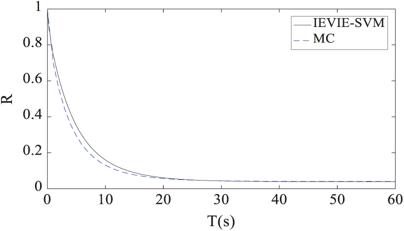
Figure 1: Comparison between the IEVIE-SA and MC methods for the case of
Fig. 2a shows the results when the number of pedestrians was
Fig. 3 shows stability reliability when the frequency ratio was fixed and the number of pedestrians was varied. Fig. 3a corresponds to the case of
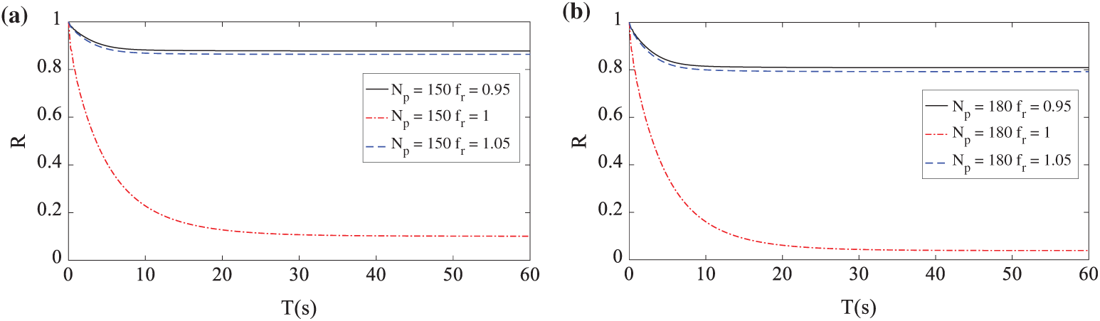
Figure 2: Stability reliability with a fixed number of pedestrians and the variant frequency ratio:
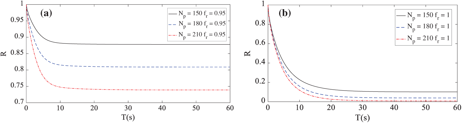
Figure 3: Stability reliability under a fixed frequency ratio and varying numbers of pedestrians: (a)
To more clearly illustrate the influence of parameters on vibrational stability, Fig. 4 shows a three-dimensional diagram of stability reliability under different combinations of pedestrian number and frequency ratios. The shape of the surface of
Of note, compared with the traditional Lyapunov method that can only obtain two qualitative results (stability or instability), the quantitative results obtained by the proposed method contained more information and were more practical, especially for designers.
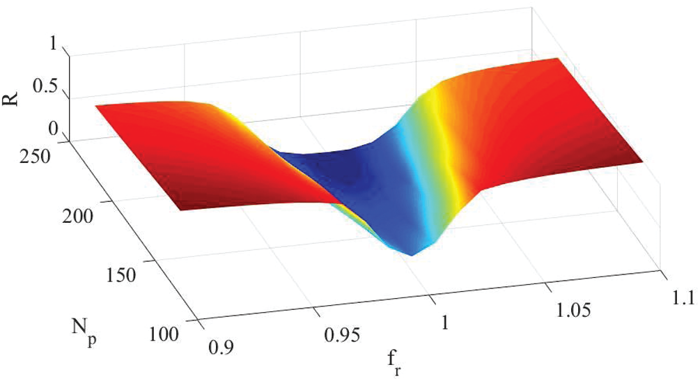
Figure 4: Three-dimensional graph of
The influence of randomness on the system stability is also investigated through the parameter analysis of
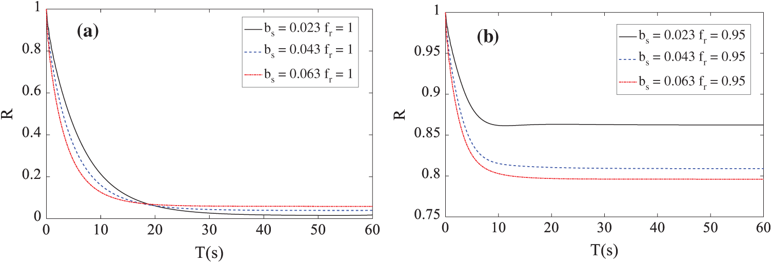
Figure 5: Stability reliability with different combinations of
To further verify the effectiveness of the proposed method, the Lyapunov method based on the maximal Lyapunov exponent was implemented for comparison. Performing a linear operation about the derived coefficients in Eq. (27) at
With
Since
In addition,
where
where
The stability of the trivial solution of Eq. (38) was determined by the sign of
Unlike the traditional Lyapunov definition of random vibrational stability, we can simply give the definition of random vibrational stability according to the probability obtained from IEVIE-SA. If the following equation was satisfied,
the system was stable with probability
Fig. 6 compares the results of the
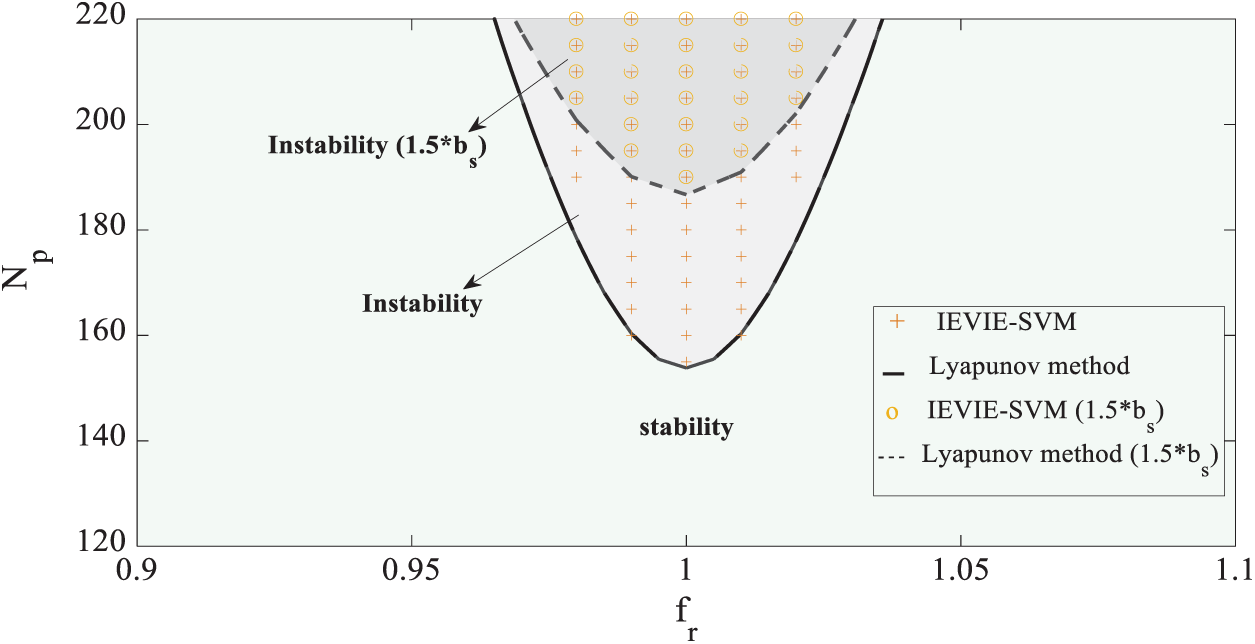
Figure 6: Comparison of the IEVIE-SA and Lyapunov methods
This study established a framework to efficiently and quantitatively analyze the stability reliability of the lateral vibration of a footbridge. The IN model was used to describe the lateral vibration of footbridges, considering the correlation between pedestrian excitation and bridge vibration, and the randomness of pedestrian excitation. The IEVIE method based on the comparison of input energy and the variation of intrinsic energy was used to establish the judging criteria to identify vibrational stability. In addition, the SA method was used to establish the stochastic Itô equation with slow variables as well as the corresponding backward Kolmogorov equation for condition reliability. Subsequently, the stability criterion established by the IEVIE was combined and treated as the boundary condition of the first passage reliability within the backward Kolmogorov equation, by which the first passage reliability of vibrational stability was obtained. The main results were as follows:
1) The proposed method was successfully applied to the central span of the Millennium Bridge, and its validity was verified by comparing it with the MC and traditional Lyapunov methods.
2) The frequency had an important influence on the lateral vibrational stability of the footbridge. When the walking frequency was equal to the doubled bridge frequency, stability reliability had an extremely small probability. This may explain the large vibration of the central span of the Millennium Bridge, which has a fundamental frequency that is half of the pedestrian walking frequency. The number of pedestrians also affected the lateral vibrational stability of the footbridge. Stability reliability decreased with increasing numbers of pedestrians. When the number of pedestrians reached 180 under the worst case (
3) Compared to the number of pedestrians, the frequency had a more dominant influence on the lateral vibrational stability of the footbridge. However, the influence from the number of pedestrians and the frequency were coupled: the greater the number of pedestrians, the more frequency points that could cause a large probability of instability. On the other hand, the closer the frequency ratio was to 1, the greater the change in stability reliability caused by the number of pedestrians.
4) Compared to the traditional Lyapunov method, the proposed method could conduct quantitative analysis of the random vibrational stability of the footbridge, which is more practical and reasonable. Another advantage of the proposed method is that it uses the stochastic averaging method to simplify the stochastic equations, which greatly reduces the number of calculations.
Nevertheless, the proposed method also has some limitations. First, the IN model used in this study was essentially a backstepping model and did not guarantee that the full mechanism of the lateral vibration of the footbridge was revealed. In the future, more valuable data should be collected to further refine this model. Second, in this study, only three parameters were analyzed: the number of pedestrians, the frequency ratio, and the intensity of random disturbances. There may be other key parameters that also have an important influence on the lateral vibrational stability of the footbridge. Therefore, more detailed studies with respect to parametric analysis are needed. Third, for the sake of simplicity, this paper considers only the first-order mode, thus the suitability of the proposed method in another adjacent mode (e.g., the lateral second mode with a frequency around 1 Hz in the central span of the Millennium Bridge) cannot be guaranteed. Moreover, it cannot exclude the possibility that the forced resonance and subharmonic resonance may act simultaneously to drive the large lateral vibration, which is worth studying in the future. Finally, due to the limited data, this study only used the Millennium Bridge as a numerical example. It is necessary to collect information from other footbridges as references to further verify the generality of the proposed method.
Funding Statement: This research was supported by the National Natural Science Foundation of China (No. 51608207) and the Natural Science Foundation of Guangdong Province, China (No. 2019A1515011941).
Conflicts of Interest: The authors declare that they have no conflicts of interest to report regarding the present study.
1. Pedersen, L., Frier, C. (2010). Sensitivity of footbridge vibrations to stochastic walking parameters. Journal of Sound and Vibration, 329(13), 2683–2701. DOI 10.1016/j.jsv.2009.12.022. [Google Scholar] [CrossRef]
2. Fujino, Y., Siringoringo, D. M. (2016). A conceptual review of pedestrian-induced lateral vibration and crowd synchronization problem on footbridges. Journal of Bridge Engineering, 21(8), C4015001. DOI 10.1061/(ASCE)BE.1943-5592.0000822. [Google Scholar] [CrossRef]
3. Dallard, P., Fitzpatrick, T., Flint, A., Low, A., Smith, R. R. et al. (2001). London Millennium Bridge: Pedestrian-induced lateral vibration. Journal of Bridge Engineering, 6(6), 412–417. DOI 10.1061/(ASCE)1084-0702(2001)6:6(412). [Google Scholar] [CrossRef]
4. Hoorpah, W., Flamand, O., Cespedes, X. (2008). The simon de beauvoir footbridge in Paris. Experimental Verification of the dynamic behaviour under pedestrian loads and discussion of corrective modifications. Proceedings of Footbridge. Porto. [Google Scholar]
5. Brownjohn, J. M. W., Fok, P., Roche, M., Moyo, P. (2004). Long span steel pedestrian bridge at Singapore Changi Airport–Part 1: Prediction of vibration serviceability problems. Structural Engineer, 82(16), 21–27. [Google Scholar]
6. Brownjohn, J. M. W., Fok, P., Roche, M., Omenzetter, P. (2004). Long span steel pedestrian bridge at Singapore Changi Airport–Part 2: Crowd loading tests and vibration mitigation measures. Structural Engineer, 82(16), 28–34. [Google Scholar]
7. Racic, V., Brownjohn, J. M. W. (2011). Mathematical modelling of random narrow band lateral excitation of footbridges due to pedestrians walking. Computers & Structures, 90–91(1), 116–130. DOI 10.1016/j.compstruc.2011.10.002. [Google Scholar] [CrossRef]
8. Racic, V., Brownjohn, J. M. W. (2011). Stochastic model of near-periodic vertical loads due to humans walking. Advanced Engineering Informatics, 25(2), 259–275. DOI 10.1016/j.aei.2010.07.004. [Google Scholar] [CrossRef]
9. Nakamura, S. (2004). Model for lateral excitation of footbridges by synchronous walking. Journal of Structural Engineering, 130(1), 32–37. DOI 10.1061/(ASCE)0733-9445(2004)130:1(32). [Google Scholar] [CrossRef]
10. Piccardo, G., Tubino, F. (2008). Parametric resonance of flexible footbridges under crowd-induced lateral excitation. Journal of Sound & Vibration, 311(1–2), 353–371. DOI 10.1016/j.jsv.2007.09.008. [Google Scholar] [CrossRef]
11. Ingólfsson, E. T., Georgakis, C. T., Ricciardelli, F., Jönsson, J. (2012). Experimental identification of pedestrian-induced lateral forces on footbridges. Journal of Sound & Vibration, 330(6), 1265–1284. DOI 10.1016/j.jsv.2010.09.034. [Google Scholar] [CrossRef]
12. Macdonald, J. H. G. (2009). Lateral excitation of bridges by balancing pedestrians. Proceedings of the Royal Society A Mathematical Physical & Engineering Sciences, 465(2104), 1055–1073. DOI 10.1098/rspa.2008.0367. [Google Scholar] [CrossRef]
13. Ingólfsson, E. T., Georgakis, C. T. (2011). A Stochastic load model for pedestrian-induced lateral forces on footbridges. Engineering Structures, 33(12), 3454–3470. DOI 10.1016/j.engstruct.2011.07.009. [Google Scholar] [CrossRef]
14. Bocian, M., Macdonald, J., Burn, J. (2014). Probabilistic criteria for lateral dynamic stability of bridges under crowd loading. Computers & Structures, 136(16), 108–119. DOI 10.1016/j.compstruc.2014.02.003. [Google Scholar] [CrossRef]
15. Jia, B. Y., Yu, X. L., Yan, Q. S., Zheng, Y. (2017). Nonlinear stochastic analysis for lateral vibration of footbridge under pedestrian narrowband excitation. Mathematical Problems in Engineering, 2017(22), 1–12. DOI 10.1155/2017/5967491. [Google Scholar] [CrossRef]
16. Jia, B. Y., Yu, X. L., Yan, Q. S. (2018). Effects of stochastic excitation and phase lag of pedestrians on lateral vibration of footbridges. International Journal of Structural Stability & Dynamics, 18(7), 1–17. DOI 10.1142/S0219455418500955. [Google Scholar] [CrossRef]
17. Nawrotzki, P., Eller, C. (2000). Numerical stability analysis in structural dynamics. Computer Methods in Applied Mechanics and Engineering, 189(3), 915–929. DOI 10.1016/S0045-7825(99)00407-7. [Google Scholar] [CrossRef]
18. Ziegler, H. (1977). Principles of structural stability. Basel: Birkhauser. [Google Scholar]
19. La Salle, J., Lefschetz, S. (2012). Stability by Liapunov's direct method with applications by Joseph L Salle and Solomon Lefschetz. New York: Elsevier. [Google Scholar]
20. Zhu, W. Q. (1992). Nonlinear stochastic dynamics and control—Hamiltonian theoretical framework. Beijing: Science Press. [Google Scholar]
21. Xie, W. C. (2003). Moment Lyapunov exponents of a two-dimensional system under bounded noise parametric excitation. Journal of Sound and Vibration, 263(3), 593–616. DOI 10.1016/S0022-460X(02)01068-4. [Google Scholar] [CrossRef]
22. Wang, R., Ru, C. (1985). An energy criterion for the dynamic plastic buckling of circular cylinders under impulsive loading. New York: Elsevier. [Google Scholar]
23. Li, Y. C., Wang, Z. (2016). Unstable characteristics of two-dimensional parametric sloshing in various shape tanks: Theoretical and experimental analyses. Journal of Vibration and Control, 22(19), 4025–4046. DOI 10.1177/1077546315570716. [Google Scholar] [CrossRef]
24. Li, J., Xu, J. (2016). A quantitative approach to stochastic dynamic stability of structures. Chinese Journal of Theoretical and Applied Mechanics, 48(3), 702–713. DOI 10.6052/0459-1879-15-304. [Google Scholar] [CrossRef]
25. Xu, J., Li, J. (2015). An energetic criterion for dynamic instability of structures under arbitrary excitations. International Journal of Structural Stability and Dynamics, 15(2), 2496–2606. DOI 10.1142/S0219455414500436. [Google Scholar] [CrossRef]
26. Yuan, X. B. (2006). Research on pedestrian-induced vibration of footbridge (Ph.D. Thesis). Tongji University. Shanghai, China. [Google Scholar]
27. Brownjohn, J. M. W., Pavic, A., Omenzetter, P. (2004). A spectral density approach for modelling continuous vertical forces on pedestrian structures due to walking. Canadian Journal of Civil Engineering, 31(1), 65–77. DOI 10.1139/l03-072. [Google Scholar] [CrossRef]
28. Fujino, Y., Pacheco, B. M., Nakamura, S. I., Warnitchai, P. (1993). Synchronization of human walking observed during lateral vibration of a congested pedestrian bridge. Earthquake Engineering and Structural Dynamics, 22(9), 741–758. DOI 10.1002/eqe.4290220902. [Google Scholar] [CrossRef]
29. Ricciardelli, F., Pizzimenti, A. D. (2007). Lateral walking-induced forces on footbridges. Journal of Bridge Engineering, 12(6), 677–688. DOI 10.1061/(ASCE)1084-0702(2007)12:6(677). [Google Scholar] [CrossRef]
30. Dallard, P., Fitzpatrick, T., Flint, A., Bourva, S. L., Low, A. et al. (2001). The London millennium footbridge. Structural Engineer, 79(171), 17–33. [Google Scholar]
Appendix A: Peaceman–Rachford’s Alternate Direction Implicit Format
The two-dimensional partial differential Eq. (33) can be solved using the finite difference method. When the convergent condition is strict, the backward Euler and Crank–Nicolson schemes can be used because they are unconditionally stable. However, in these two methods, the difference equations on each time layer will have a huge number, and they are no longer tridiagonal linear equations. The calculations for solving such equations are unacceptable. In this study, the Peaceman–Rachford’s alternate direction implicit format (PR ADI) was used, and PR ADI was unconditionally stable and could be solved using the chasing method. For convenience,
where
By setting λ values as
Eq. (A1) could be rearranged as
The matrix form corresponding to Eq. (A1) had the following form:
By combining the initial condition (Eq. (34)) and the boundary conditions (Eqs. (35) and (36)) and using the chasing method to solve Eq. (A4), the solution of
The matrix form corresponding to Eq. (A5) can be expressed as
Like that for Eq. (A4), the chasing method can be used to solve Eq. (A6) to obtain the result of the
 | This work is licensed under a Creative Commons Attribution 4.0 International License, which permits unrestricted use, distribution, and reproduction in any medium, provided the original work is properly cited. |