| Computer Modeling in Engineering & Sciences |
DOI: 10.32604/cmes.2021.014993
ARTICLE
An Improved Algorithm for the Detection of Fastening Targets Based on Machine Vision
College of Nuclear Technology and Automation Engineering, Sichuan Key Laboratory of Geoscience Nuclear Technology, Chengdu University of Technology, Chengdu, 610059, China
*Corresponding Author: Haihui Huang. Email: hhh925475@163.com
#These authors contributed equally to this work.
Received: 14 November 2020; Accepted: 31 March 2021
Abstract: Object detection plays an important role in the sorting process of mechanical fasteners. Although object detection has been studied for many years, it has always been an industrial problem. Edge-based model matching is only suitable for a small range of illumination changes, and the matching accuracy is low. The optical flow method and the difference method are sensitive to noise and light, and camshift tracking is less effective in complex backgrounds. In this paper, an improved target detection method based on YOLOv3-tiny is proposed. The redundant regression box generated by the prediction network is filtered by soft nonmaximum suppression (NMS) instead of the hard decision NMS algorithm. This not only increases the size of the network structure by 52 × 52 and improves the detection accuracy of small targets but also uses the basic structure block MobileNetv2 in the feature extraction network, which enhances the feature extraction ability with the increased network layer and improves network performance. The experimental results show that the improved YOLOv3-tiny target detection algorithm improves the detection ability of bolts, nuts, screws and gaskets. The accuracy of a single type has been improved, which shows that the network greatly enhances the ability to learn objects with slightly complex features. The detection result of single shape features is slightly improved, which is higher than the recognition accuracy of other types. The average accuracy is increased from 0.813 to 0.839, an increase of two percentage points. The recall rate is increased from 0.804 to 0.821.
Keywords: Deep learning; target detection; YOLOv3-tiny
According to a survey, the global automotive fastener market is expected to grow by 4 billion US dollars, with an increase rate of 2.6%. In many developed countries, the demand for fasteners is more apparent. For example, the United States will maintain a 3.2% growth momentum. In the next five to six years, Germany will increase investment by 212 million US dollars. To date, the fastener market in Japan is 952.9 million US dollars. As the second largest economy in the world, the growth potential of China is 2.4% [1]. Therefore, in the everchanging fastener market, it is particularly important to continuously improve fastener sorting technology.
In recent years, deep convolutional networks have made breakthrough progress in various fields. A deep convolutional network mainly deepens the network level by a weight sharing strategy so that the network has a stronger analysis ability. Hamdia et al. developed a deep neural network (DNN) model to evaluate the flexoelectric effect in truncated pyramid nanostructures under compression conditions [2].
Guo et al. [3] proposed a depth allocation method (DCM) based on a feedforward DNN. Anitescu et al. [4]. proposed a method for solving partial differential equations with artificial neural networks and an adaptive configuration strategy. This method is completely meshless because only scattered point sets are used in training sets and evaluation sets, and it shows good accuracy results for the selected parameters. In the field of part identification, Wang et al. [5] developed a CNN-based visual sorting system with cloud-edge computing for flexible manufacturing systems.
In actual production, due to variabilities in the assembly process and unsystematic parts management, a large number of fasteners with different specifications are mixed together, which greatly reduces the efficiency and accuracy of subsequent assembly production. It is of great practical significance to accurately separate these artifacts.
Target detection technology is a core technology of vision systems, including target recognition and target location technology [6]. A traditional target detection algorithm consists of three parts: region selection, feature extraction and a classifier. First, the image is selected by a sliding window. Second, the selected region is extracted by an artificially designed feature extractor. Finally, a classifier is used for classification [7]. Traditional machine vision target detection mainly uses and improves the optimization of a local binary pattern (LBP)/Harr/histogram of oriented grids (HOG)+support vector machines (SVM)/AdaBoost and other algorithms [8]. Fig. 1 shows a traditional target detection flow chart.

Figure 1: Traditional target detection flow chart
In the research of Wren et al. [9], it was found that although the traditional target detection algorithm is simple, intuitive and relatively fast, the design of the feature extractor depends on the designer's experience, which can only extract local shallow features of the image but cannot extract the abstract features of the image. At the same time, the application of anti-interference ability is very poor in complex scenes.
In recent years, with the maturity of GPU technology, deep learning has developed rapidly. With the development of GPU technology, the development of neural networks has been promoted. In most cases, the formation of deep learning models without graphics processors is very slow [10]. At present, target detection algorithms based on deep learning can be divided into two categories: one is based on candidate regions (two-stage), and the other is based on regression target detection (single-stage) [11].
The target sorting method based on a candidate box is a two-stage detection method that generates a suggestion box and classifies and regresses the objects in the suggestion box to generate the final results. In recent years, many researchers have performed much research on target detection using this method. In 2014, Girshick et al. [12] proposed the regional convolutional neural network (R-CNN) to successfully apply deep learning to the field of target detection. The algorithm mainly includes regional nomination, normalization, feature extraction, classification and regression. Although the structure of the R-CNN target detection framework is similar to that of the traditional detection framework, the convolutional neural network (CNN) has a stronger feature extraction ability than traditional HOG feature extraction methods. The final result of the pattern analysis, statistical modeling and computational learning visual object classes (Pascal VOC) data set reaches 53.7%, while the accuracy of the traditional feature extraction method can only reach approximately 34.3%. Girshick [13] of the Microsoft Research Institute proposed the Fast R-CNN algorithm in 2015. The algorithm designed a region of interest (ROI) pooling structure according to the spatial pyramid pooling network (SPP-Net) pyramid pooling method, which better solved the time consumption caused by the normalization operation in the R-CNN. Ren et al. [14] of the Microsoft Research Institute put forward the Faster R-CNN algorithm, realized the two-stage structure of the whole network, and designed a new region proposal network (RPN) module to replace the traditional selective search module, which effectively avoids the problem of a large calculation amount caused by generating too many candidate frames.
A target detection algorithm based on regression obtains the detection position and category directly through the whole picture, and the representative algorithms are the You Only Look Once (YOLO) series. In 2016, Redmon of Washington University proposed the YOLO algorithm, which directly expanded the original image to 448 × 448 and divided it into 7 × 7 grids [15]. The whole image was directly input into a convolutional neural network for feature extraction training, and the results were generated in each divided grid by frame regression and category judgment, which greatly improved the detection speed. In December 2016, Liu of the University of North Carolina at Chapel Hill proposed the single-shot multibox detector (SSD) algorithm, which combined YOLO with the RPN anchor mechanism in Faster R-CNN and used frames of different sizes and proportions to regress at different positions on the whole picture, finally improving the detection accuracy while maintaining a high detection speed [16]. The YOLOv3 algorithm was proposed by Redmon et al. [17] in 2018. Compared with the YOLOv1, YOLOv2 and SSD versions, YOLOv3 has the highest detection accuracy and better real-time performance and has become the most commonly used target detection framework in engineering. However, YOLOv3-tiny is also one of our important choices for projects with high speed requirements, limited experimental equipment and high pairs of positive and negative samples. YOLOv3-tiny is a lightweight model in YOLOv3 that greatly accelerates the detection speed by simplifying the complexity of the network model and keeping two prediction branches [18].
The algorithms in the above documents still have some shortcomings, such as slow detection speed, large consumption of network resources, low accuracy and recall rate, and poor detection accuracy. In this paper, we use deep learning technology to realize target detection. In view of the simple background and clear target feature pairs, this paper adopts lightweight YOLOv3-tiny as the basic detection framework and improves it to realize target detection. This model is simple in structure and low in computational complexity and can be run on a mobile terminal and a device terminal. Experimental results show that this algorithm has high detection accuracy and robustness in target detection.
2 Target Detection Algorithm Based on YOLOv3
2.1 YOLOv3-Tiny Network Structure
As shown in Fig. 2, the network structure of YOLOv3-tiny consists of seven convolutional layers and five maximum pooling layers, which are mainly composed of a series of convolutions, and the convolution kernel size is 3 ∗ 3. When the size of the network input is 416 ∗ 416, the size of the output characteristic graph becomes 1/2 of the original size for each maximum pooling operation. After five maximum pooling operations, the size of the feature image becomes 1/32 of that of the original image [19].
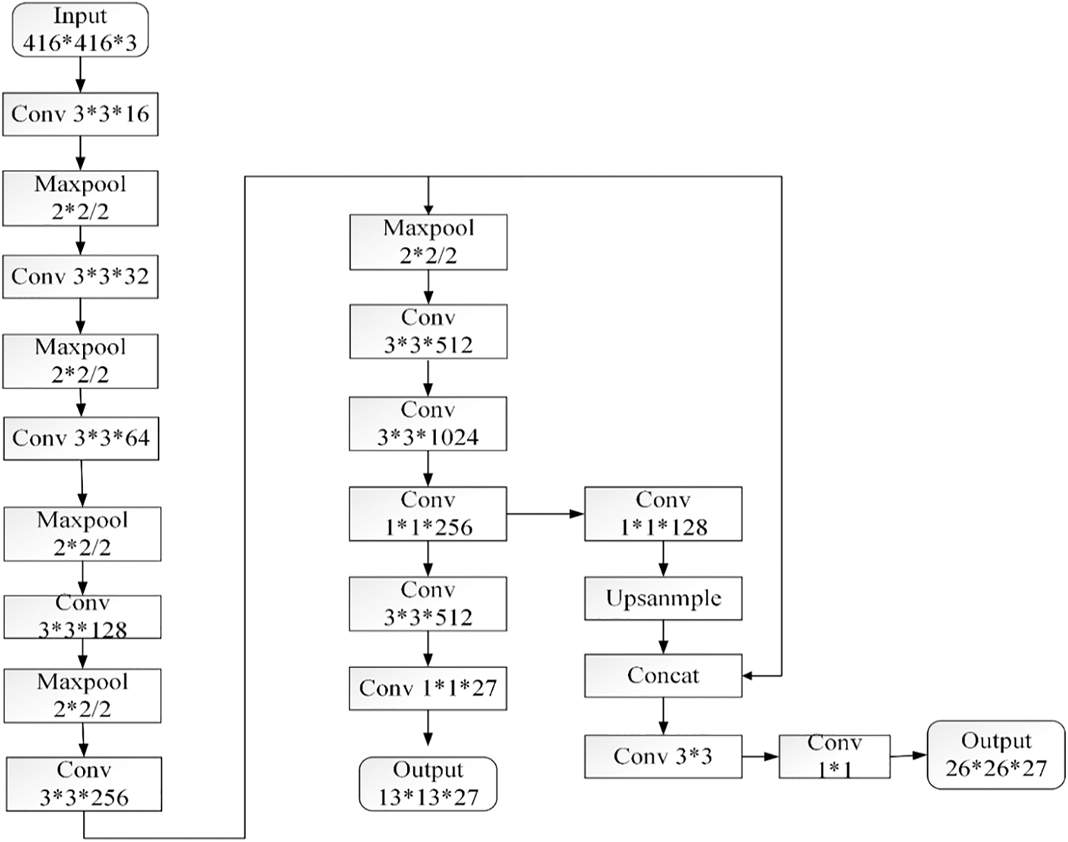
Figure 2: YOLOv3-tiny network structure
As shown in Fig. 2, to solve the problem of low accuracy in single-scale target detection, YOLOv3-tiny adopts two scale prediction methods, taking the input picture size of 416 ∗ 416 as an example, and finally generates feature layers with scales of 13 ∗ 13 and 26 ∗ 26. YOLOv3-tiny sets three prior frames for each scale, with a total of six anchor boxes for prior frames of different sizes. The minimum scale feature map is 13 ∗ 13, that is, 32 downsamplings, and the corresponding perceptual field on the original map is 32 ∗ 32. Therefore, a larger prior frame should be used to detect the larger image. A feature map with a scale of 26 ∗ 26, i.e., 16 downsamplings, is implemented, and the corresponding perceptual field on the original map is 16 ∗ 16, so it is necessary to use a smaller prior box to detect small and medium objects. Each grid of each scale feature image outputs a tensor with a depth of 3 ∗ (1 + 4 + C), and each grid has three tasks. First, confidence is used to determine whether there is a target object in the grid. Second, the center point of the output frame is offset. Finally, the classification of the target is determined.
YOLOv3-tiny is initialized by using the prior box obtained by the anchor mechanism. YOLOv3-tiny predicts the offset between the center point of the boundary and the upper left corner of the corresponding grid [20]. The transition between the predicted value and the true value of the frame is shown in Fig. 3.
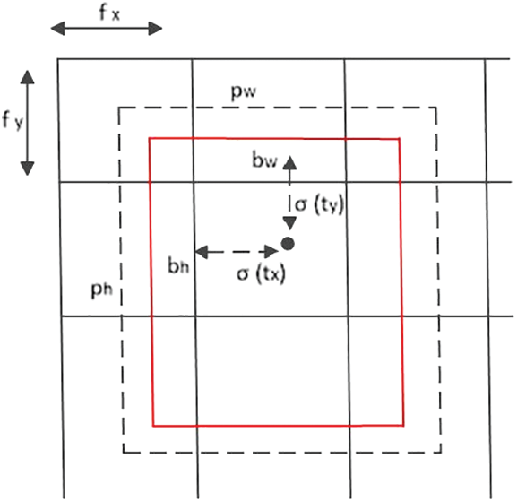
Figure 3: Conversion diagram of the predicted value and real value of the bounding box
In Eq. (1), tx, ty, tw and th are network prediction values for each frame. It predicts the offset between the center of the bounding box and the upper left corner of the target grid cell. bx, by, bw, and bh are the predicted coordinate values. fx and fy are the offset values of the upper left corner of the grid, where the center point is relative to the upper left corner of the original image. pw and ph are the width and height of the prior frame, respectively. The center point offset tx and ty of the prediction frame are normalized by the sigmoid function. Therefore, the coordinate conversion formula of the bounding box is shown in Eq. (1):
Nonmaximum Suppression, also known as the NMS algorithm, keeps the local maximum and suppresses the nonmaximum value [21]. It can be seen in Fig. 4 that when using the target detection algorithm, the same target predicts a large number of different candidate boxes and the confidence level of the corresponding target [22]. The candidate boxes may overlap each other. At this point, it is necessary to use nonmaximum suppression to find the best target boundary box and eliminate redundant boundaries.
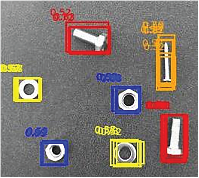
Figure 4: Target detection results without NMS
Intersection over union (IOU) is an index used to measure the degree of overlap between two prediction bounding boxes. It calculates the ratio of the intersection area and the joint area between the predicted boundary and the actual boundary. A schematic diagram is shown in Fig. 5, and its expression is shown in Eq. (2), where box1 and box2 are rectangular borders [23]:
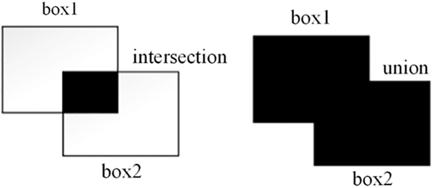
Figure 5: Schematic diagram of border intersection and union
The flow of the NMS algorithm is as shown in Fig. 6. First, the predicted rectangular boxes are sorted according to the confidence level, and the candidate frames with the highest confidence level are reserved. Then, the IOU of the remaining candidate frames and the candidate frames with the highest confidence is calculated, and it is judged whether the IOU is larger than the set threshold value T. The above process is repeated until all frames are processed.
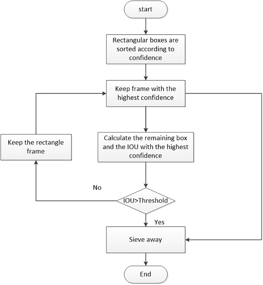
Figure 6: Nonmaximum suppression diagram
2.5 Cluster Labeling Information Box Based on the K-Means Algorithm
In the YOLOv3-tiny target detection framework, k-means clustering is used to cluster the prior box. K-means is an unsupervised learning algorithm based on distance clustering, in which k represents the number of classification categories, and means represents the average value of data samples of each category as the centroid of the category. The division is based on the nearest distance between data sample points and the centroid of each category, that is, to minimize Eq. (3) [24].
For data set clustering, the k-means algorithm is implemented as follows:
(1) Randomly generate k central points as k centroids;
(2) The Euclidean distance from each sample point to K center points is calculated, and the point is divided into the class with the smallest Euclidean distance;
(3) According to the second step, redivide the centroid of sample points;
(4) Determine whether the distance is reduced according to Eq. (3); if so, repeat Steps 2 and 3; otherwise, terminate iteration.
Figs. 7 and 8 show that the k-means algorithm classifies 6 and 9 on the data set in this paper, and the 6 classifications served serve as 2 scales and 6 suggestion boxes of YOLOv 3-tiny, among which 3 suggestion boxes corresponding to 13 scales are (36.63, 34.05), (63.16, 21.1), and (51.37, 63.31), respectively; The three scales and nine suggestion boxes used to modify YOLOv 3-tiny are advanced, among which the three suggestion boxes corresponding to 13 scale are (71.76, 24.59), (44.34, 43.38) and (53.5, 76.07), and the three suggestion boxes corresponding to 26 scale are (42.37, 17.71):
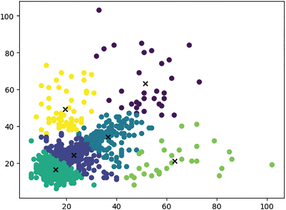
Figure 7: Six types of prior frame aggregation by k-means
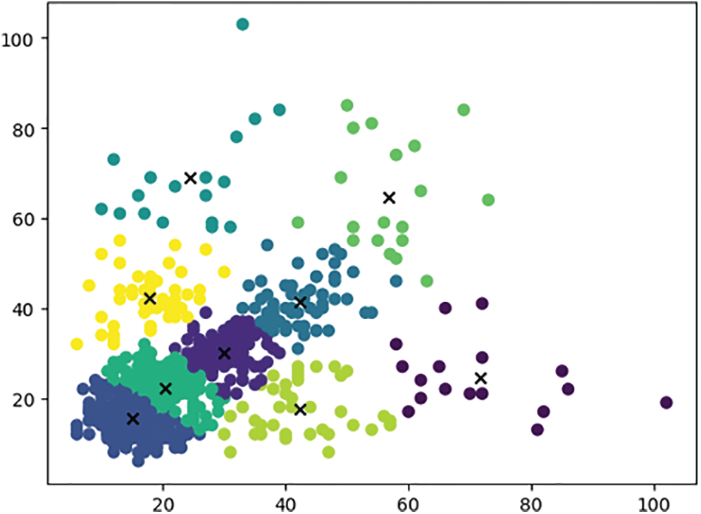
Figure 8: K-means clustering of prior frames into 9 categories
3 An Improved Target Detection Algorithm Based on YOLOv3-Tiny
3.1 Border Selection Based on Soft NMS
During the target detection process, the positions of objects tend to overlap. The YOLOv3-tiny overall network structure model predicts three frames for each grid at each scale, which generates a large number of redundant prediction frames in the network. If NMS is used as a hard decision algorithm, it is easy to delete the frames with high overlap, which can easily lead to missed detection. These problems can directly influence the performance of the model. See Section 2.4 for the algorithm flow of NMS, and see Eq. (4) for the function formula. M is the highest confidence prediction box, and bi is the i-th prediction box, which is a given threshold. It can be known from Eq. (4) that the traditional NMS exists. When the two target boxes are closed, the box with a lower score will be deleted because of the large overlap area. NMS thresholds need to be determined manually. If the setting is very small, false inspection of the assembly will be missed. Aiming at the existing problems of the NMS algorithm, a soft NMS algorithm is proposed. The soft NMS function formula is shown in Eq. (5):
The principle and steps of filtering prediction frames using soft NMS algorithms are the same as those for NMS. According to Eq. (5), the rough path of the NMS hard threshold is changed by Gaussian weighting, and the NMS algorithm is improved according to the law where the larger the IOU is, the more serious the attenuation is and the lower the confidence level is. However, the border with the overlap of the detection box with the maximum confidence level less than the threshold is not affected at reducing the possibility of false deletion, and the use of Soft-NMS for border selection does not need to retrain the model and does not increase the time cost. Fig. 9 shows the situation before and after using the NMS algorithm.
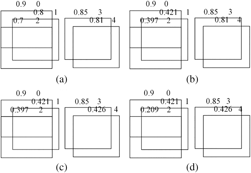
Figure 9: Comparison before and after using the NMS algorithm. (a) Original prediction frame (b) Use Soft-NMS for the first time (c) Use Soft-NMS for the second time (d) Use Soft-NMS for the third time
As shown in Fig. 9, if 0, 1, 2, 3 and 4 are the prediction boxes of adjacent objects, 0.9, 0.8, 0.7, 0.85 and 0.81 are the corresponding confidence degrees. In Fig. 9b, for the first time using the Soft-NMS algorithm to filter the prediction box, first remove the 0 box with the highest confidence and add it to the final detection results. Because the overlap degree of box 1, box 2 and box 0 with the highest confidence is larger than the set threshold, the reliability attenuation is 0.421 and 0.397, respectively, by Gaussian weighting; boxes 3 and 4 are retained directly because of the small overlap with box 0. For the remaining boxes 1, 2, 3 and 4, use the soft-NMS algorithm again. Delete the 3 boxes with the highest confidence level and add them to the final detection results. The 4 boxes that have a great overlap with the 3 boxes are attenuated to 0.426 until the iteration conditions end.
If the rough NMS algorithm is used, the IOU of prediction frames 0 and 1, 2, 3 and 4 may be too large, resulting in the last 1, 2 and 4 being considered false frames, thus deleting frames 1, 2 and 4. However, after using soft NMS, frames 1, 2 and 4 were not deleted by mistake, but their confidence was attenuated by Gaussian weighting. The higher the degree of overlap, the stronger the suppression and the worse the confidence reduction.
3.2 Improve YOLOv3-Tiny Network Structure
The YOLOv3-tiny network has a light structure and can realize target detection under limited experimental equipment conditions. However, compared with deep feature extraction networks such as darknet53, its accuracy is low. To ensure sorting accuracy, it is necessary to improve the detection accuracy of YOLOv3-tiny when the network detection meets the requirements.
Fig. 10 shows the improved network structure. The core indicators of network design are accuracy, capacity and efficiency, that is, the deeper the level, the more information fusion and the less computation. MobileNetV2 is based on the concept of MobileNetV1, which uses deep divisible convolution as an efficient building block. In addition, MobileNetV2 has introduced two new functions into the architecture. First, a 1 ∗ 1 expansion layer is added before depthwise convolution to increase the number of channels and obtain more features. Second, in point-by-point convolution, ReLU is not used, and linearity is used to prevent ReLU from destroying features. To enhance the extraction of image details, the MobileNetv2 basic convolution block and 52 ∗ 52 scale are added to the YOLOv3-tiny network, 1 ∗ 1 convolution and 3 ∗ 3 convolution are added to the third layer of the network, and 1 ∗ 1 convolution reduces half of the previous convolutional layer, making 3 ∗ 3 the computation of the convolutional layer pixel fusion reduced to half of the original, and the depth of the network deepens. The MobileNetv2 basic convolution block consists of a 1 ∗ 1 convolution, 3 ∗ 3 depth convolution and 1 ∗ 1 convolution. The first 1 ∗ 1 convolutional layer is used to increase the channel size of the feature image and fuse channels; 3 ∗ 3 depth convolution is mainly used for pixel fusion to extract features but does not fuse the channel layer; and the accumulation of the last 1 ∗ 1 convolutional block reduces the channel size of the original feature image and performs channel fusion [6]. By adding the scale of 52 ∗ 52 to the network, the corresponding perceptual field of the original image is 8 ∗ 8, which makes the improved network model enhance the detection of small targets and makes the network perform better.
The structure of the mixed domain is composed of a channel domain and a spatial domain. The attention structure of the channel domain [14] and space domain [15] is shown in Figs. 11 and 12. The significance of features is simulated in the channel domain. Maxpool and Avgpool are used for each channel, the transformation results are obtained through several convolution layers, Maxout and Avgout are superimposed, and the attention corresponding to the weight of feature estimation is generated by the sigmoid function. The importance of spatial position is modeled in the spatial domain. Maxpool and Avgpool are dimensionalized at the channel level, and then a feature graph is spliced, which is learned by a convolutional block. Then, a sigmoid function is used to generate the attention degree corresponding to the feature prediction weight. The attention mechanism in the spatial domain and channel domain is formed by generating corresponding attention weights for certain positions of the feature layer. In addition, by adding a scale of 52 ∗ 52 to the network, the visual field corresponding to the original image is 8 ∗ 8, which enhances the detection of small targets in the improved network model and improves the network performance.
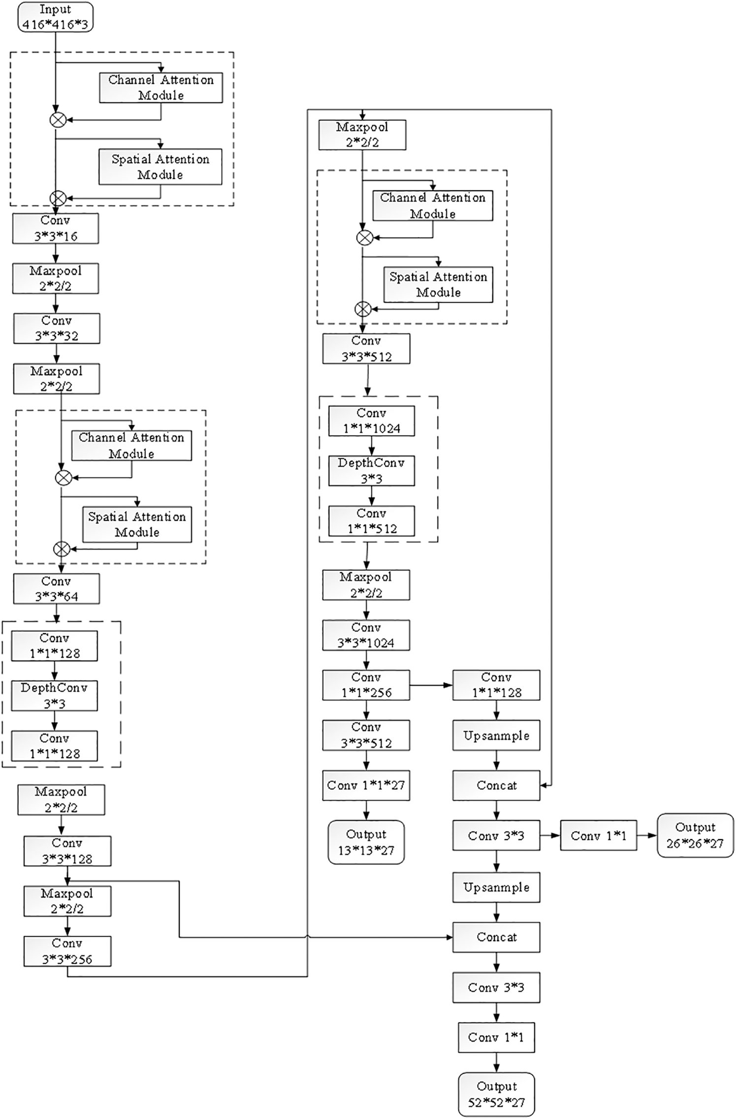
Figure 10: Improved YOLOv3-tiny network structure
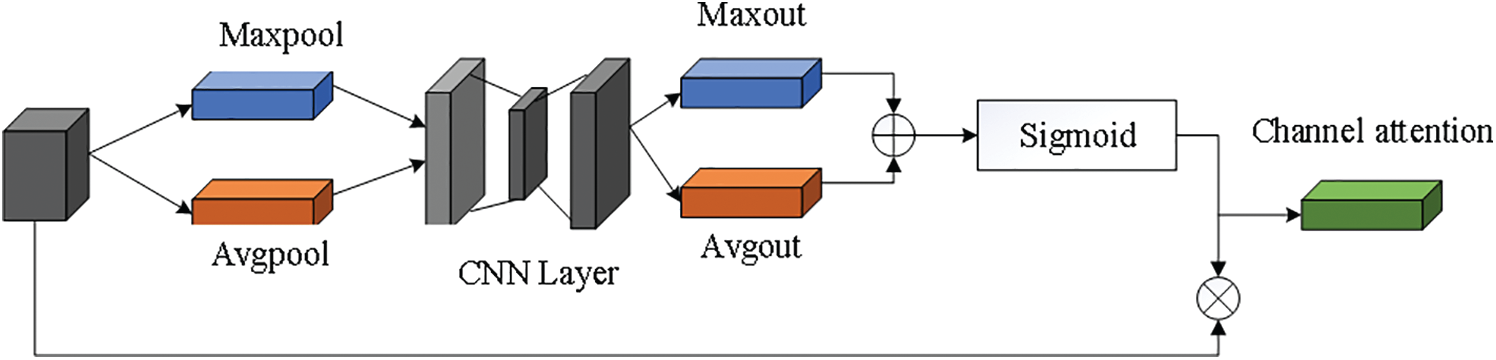
Figure 11: Channel attention module
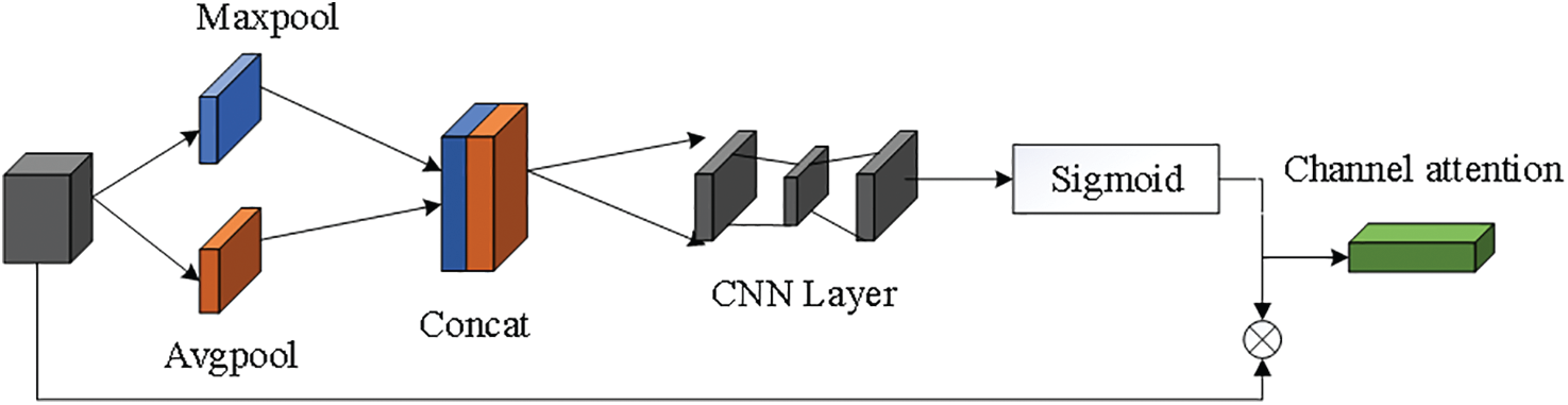
Figure 12: Spatial attention module
4.1 Software Design of Upper Computer
According to the functional requirements of the sorting system, the human-computer interaction software is compiled on the computer. The software interface is shown in Fig. 13. The software is developed based on vs2013. Its main functions include an image acquisition window, manipulator motion control, hand-eye calibration, recognition and grasping. The image acquisition window mainly includes the conventional camera opening and closing operation. The motion control mainly includes the parameter control of the four-axis manipulator, which can manually control the manipulator to reach the designated position and acquire the attitude parameters of the manipulator in real time.
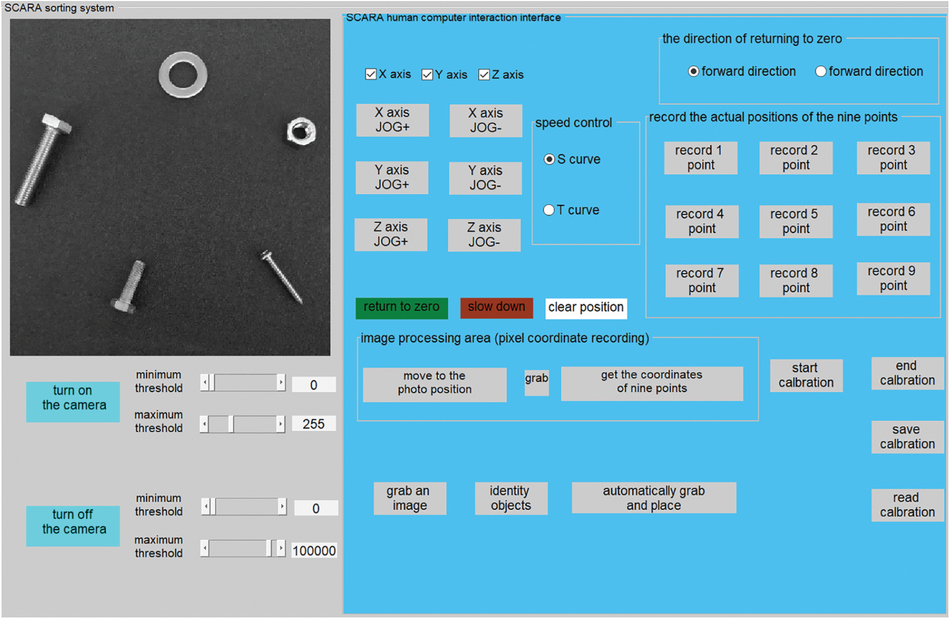
Figure 13: Robot man-machine interaction interface
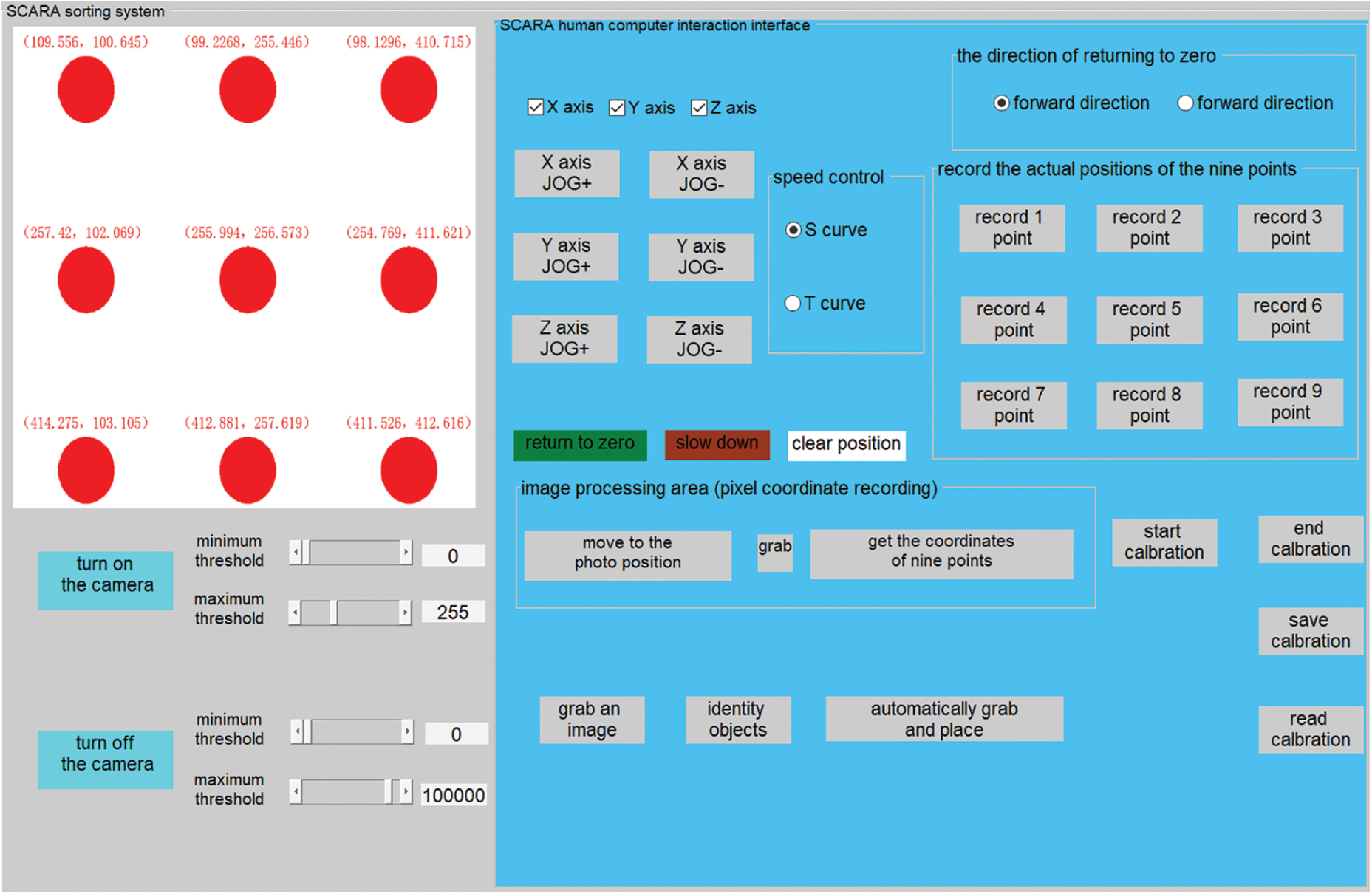
Figure 14: Hand-eye calibration of manipulator
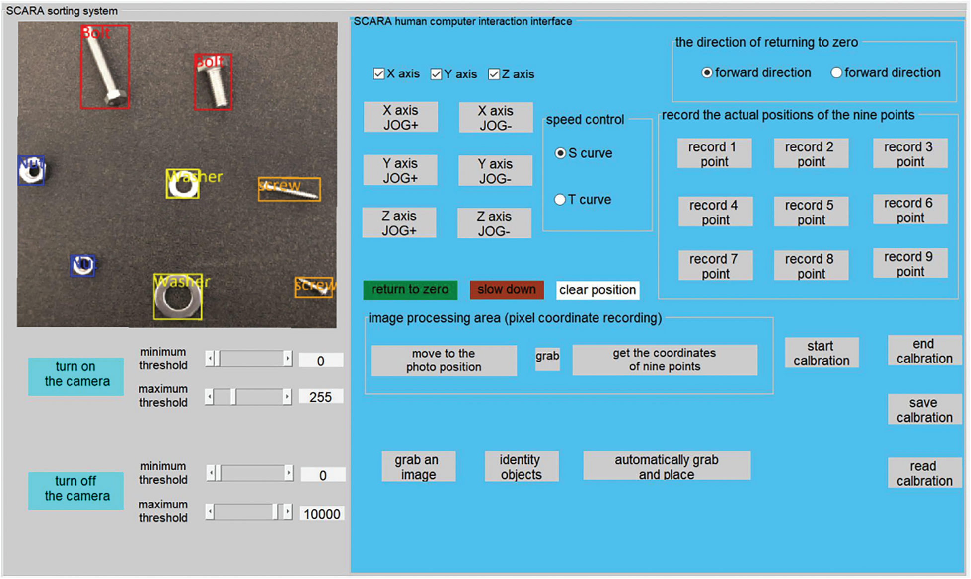
Figure 15: Positioning and recognition of fasteners
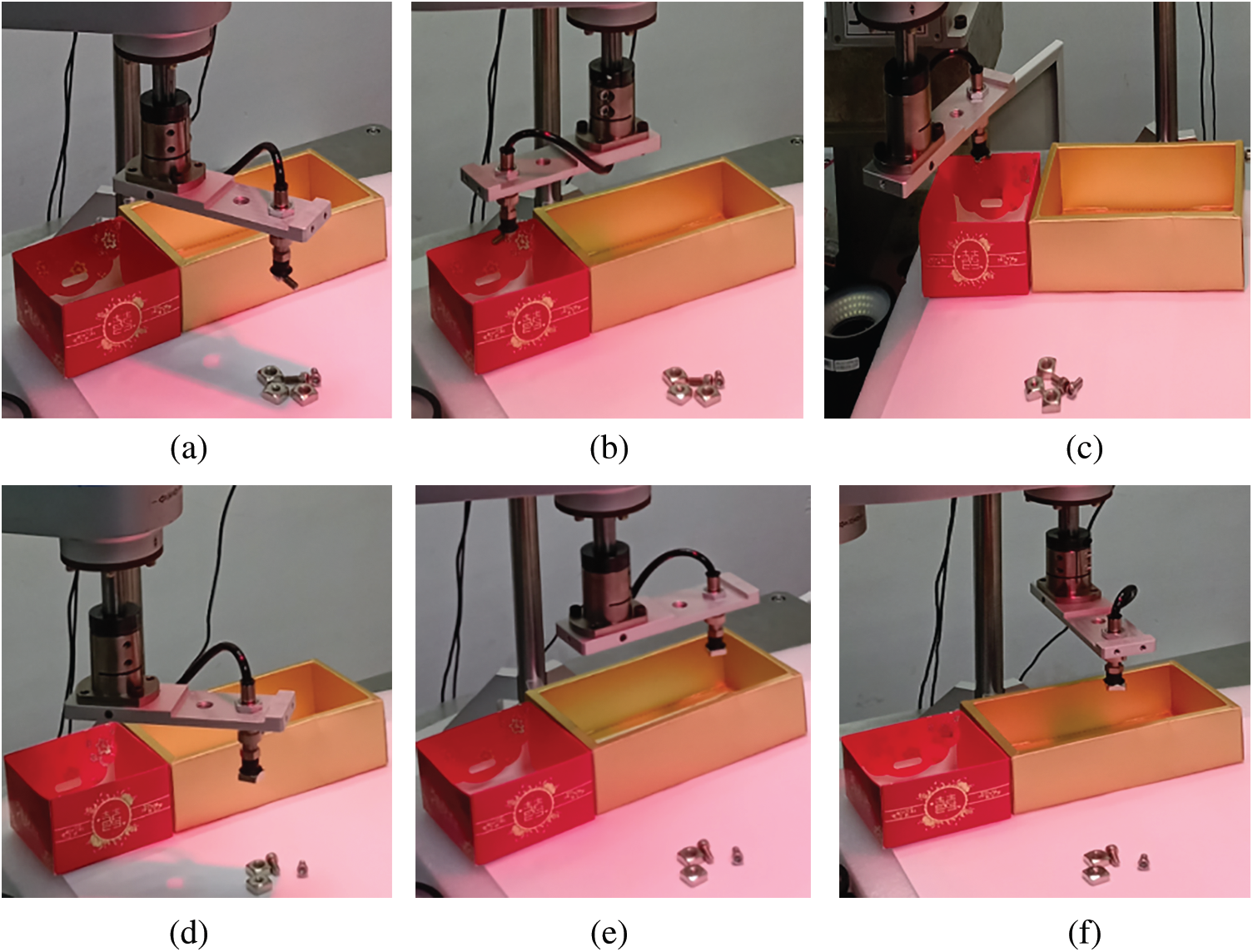
Figure 16: Grasping and sorting of fasteners (a) Grasping bolt (b) Moving bolt (c) Arrival at the designated position (d) Grasping nut (e) Moving nut (f) Arrival at the designated position
This experiment adopts a simpler nine-pointibration method, which means that the mobile manipulator locates the nine-point position point by point and records the corresponding manipulator coordinates in the hand-eyealibration module to store the nine-point manipulator coordinate records. Then, the software obtains and saves the current pixel coordinate position of the center at 9 o'clock in Fig. 14. After obtaining the pixel coordinates and manipulator coordinates, click start calibration to obtain the calibration matrix.
When calling the trained network model for target detection, the detection results of the upper computer are shown in Fig. 15. It can be seen in the figure that the center point of target positioning has a high coincidence degree with the actual center point, and the error is small, so the success rate of grabbing and sorting is high. The experimental results show that the software system can accurately identify and position fasteners.
For robot grabbing, the grabbed workpiece is placed at the designated position to finish the sorting task. The fastener grabbing and sorting experiment is shown in Fig. 16.
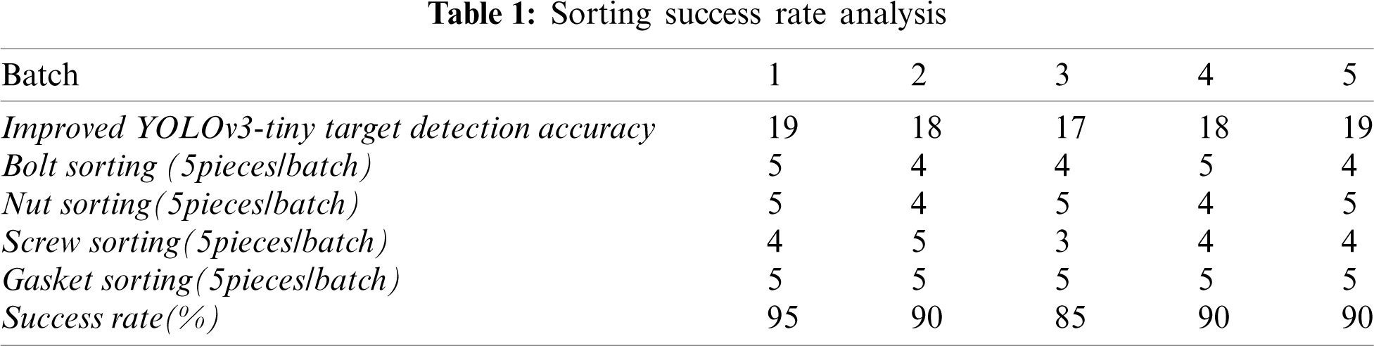
A total of 100 fasteners, including the same number of bolts, nuts, screws and washers, are uniformly mixed in 5 batches and placed in a specific area within the camera's visual field, and the number of the four fasteners successfully sorted by the robot is recorded. Tab. 1 shows the measured data results.
Training a deep network requires many parameters, but in practice, the number of training samples may be insufficient, which leads to the risk of overfitting in the network. Therefore, a large amount of data is needed to reduce this risk. The main methods for obtaining large amounts of data are to obtain a large number of new samples or to enhance the data according to the existing samples. The former has a high cost, while the latter has a low cost. On the one hand, the function of data enhancement is to improve the data volume and generalization ability of the model and, on the other hand, to improve the robustness of the model by adding various noise data. Common classification methods of data enhancement are divided into offline enhancement and online enhancement. Offline enhancement uses various methods to process data set samples before training, which is suitable for small data sets. Online enhancement processes each batch of samples during training, which is typically used for large data sets. The commonly used data enhancements include rotation, scaling, flipping, noise, color enhancement, and affine transformation. Through data enhancement, the training effect of the model is generally reduced, but the testing accuracy of the model is improved, and the labeling complexity caused by a large amount of data is reduced. By rotating, flipping, color dithering, contrast enhancement, adding Gaussian noise to each sample and rotating, the generalization ability of the sample can be improved. Fig. 17 shows part of an image after sample enhancement, where Fig. 17a shows the original image, Fig. 17b shows the image after an up-and-down flip, Fig. 17c shows the image after color jitter, Fig. 17d shows the image after contrast enhancement, Fig. 17e shows the image after adding Gaussian noise, and Fig. 17f shows the image after rotation.
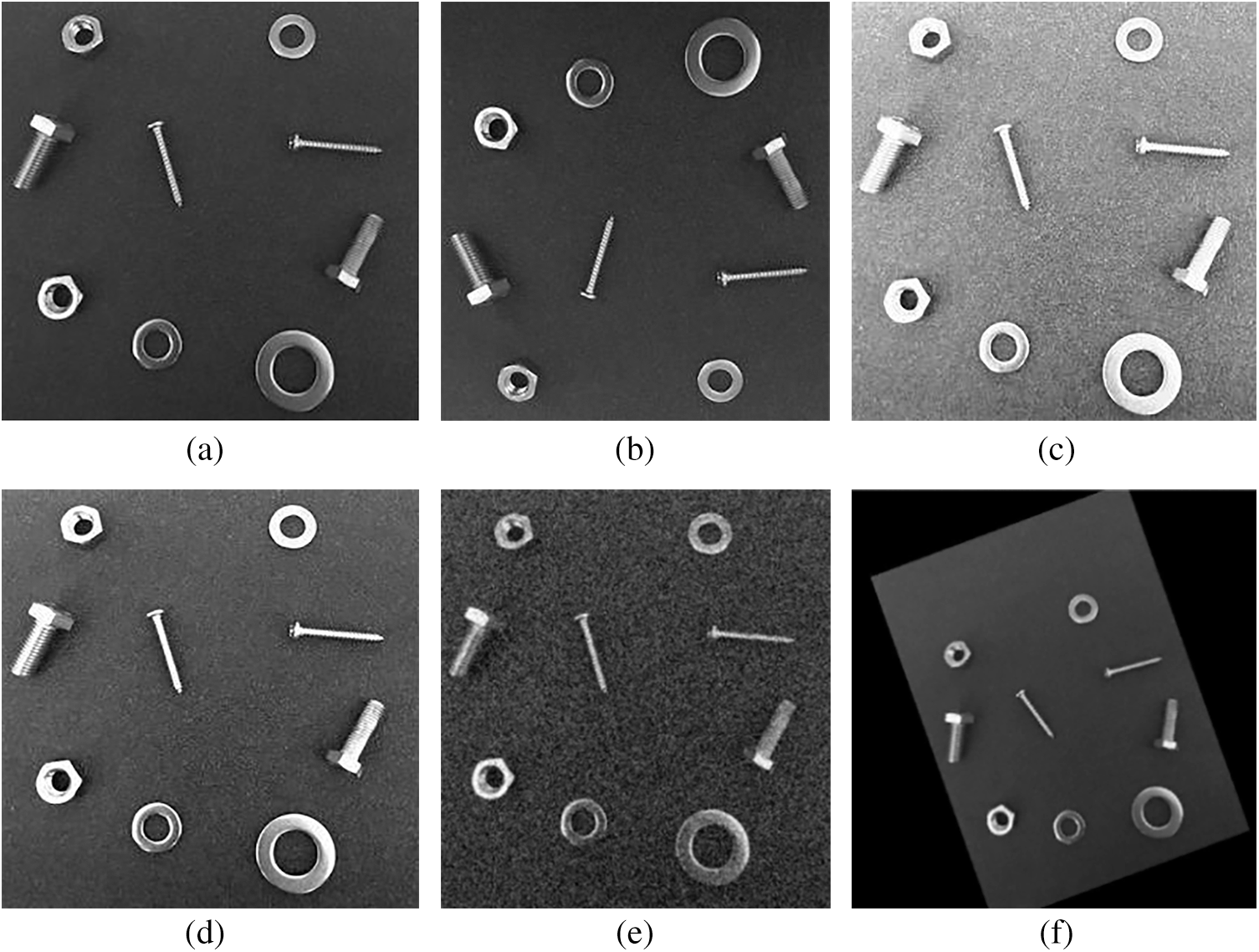
Figure 17: Image enhancement (a) Original (b) flip (c) color jitter (d) Contrast enhancement (e) plus Gaussian noise (f) rotation
4.3 Algorithmic Training Process
By labeling the assistant, the collected and enhanced training set images are manually labeled, and all the images are randomly divided into a training set and a test set at a ratio of 8:2. During the network training stage, the random gradient descent method is used to optimize the weight coefficient. After many iterations, the network weight parameters are constantly updated, YOLOv3-tiny is trained, and the target detection model is improved. The adaptive gradient (Adagrad) algorithm is very suitable for dealing with sparse data, and the root mean square Prop (RMSprop) algorithm can alleviate the problem where the learning speed of the Adagrad algorithm drops too fast. The main advantage of Adam is that the learning rate of each iteration has a certain range after offset correction so that the parameters are relatively stable. Therefore, the Adam optimization algorithm is more advantageous than RMSprop and Adagrad. Through the iterative training of 2500 batches of YOLOv3-tiny and its improved target detection model, it is found that the change in loss is stable, and the loss value is reduced to approximately 0.009 as shown in Fig. 18.
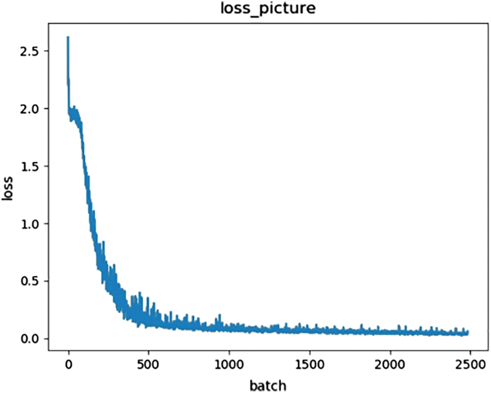
Figure 18: Training loss of improved YOLOv3-tiny
As shown in Fig. 19, after 620 rounds of verification training on the test set, it is found that the change of loss tends to be stable, and the loss value drops to approximately 0.001.
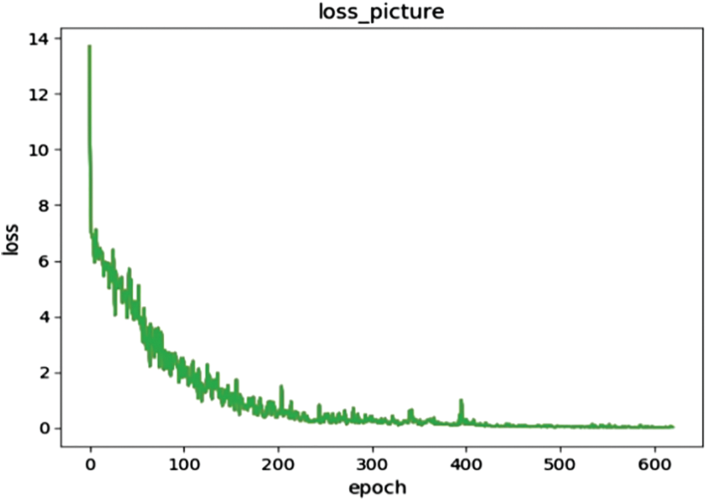
Figure 19: Validation loss of improved YOLOv3-tiny
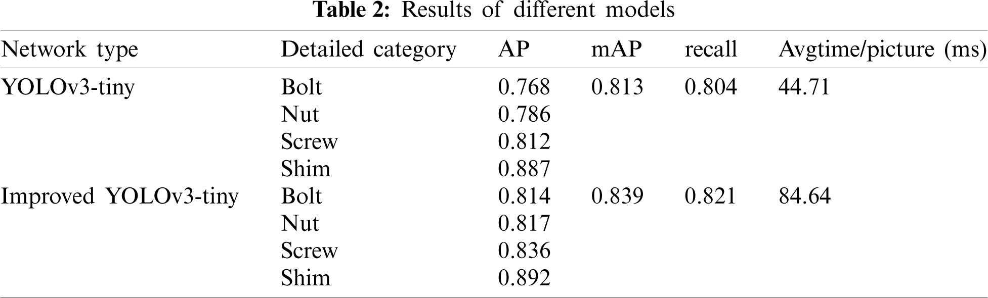
The improved YOLOv3-tiny model is consistent with the original YOLOv3-tiny training set, testing set and confidence threshold. The two networks trained on the same batch of data sets detect the target of four kinds of pictures. The confidence threshold and the soft NMS threshold are 0.6 and 0.6, respectively. After repeated training, the model parameters are adjusted to the best condition. The two models are trained with the same training samples, and the results of repeated sampling are shown in Tab. 2.
It can be seen in the above table that, compared with the detection results of the improved YOLOv3-tiny and YOLOv3-tiny networks, the improved YOLOv3-tiny network has an improved detection ability for bolts, nuts and screws, and the accuracy of a single class is improved to some extent, indicating that the network greatly enhances the ability to learn objects with slightly complex features. The results of the gasket inspection with a single shape feature improves slightly, the average accuracy rate increases from 0.813 to 0.839, which is 2 percentage points higher than other categories, and the recall rate increases from 0.804 to 0.821, which is nearly two percentage points higher. The speed and improvement of YOLOv3-tiny were tested. The average detection speed of the YOLOv3-tiny model is 44.71 milliseconds per picture. However, the improved YOLOv3-tiny reduces the detection speed and improves the accuracy due to the increase in network layers and scales. The detection speed is 84.64 ms for each picture on average.
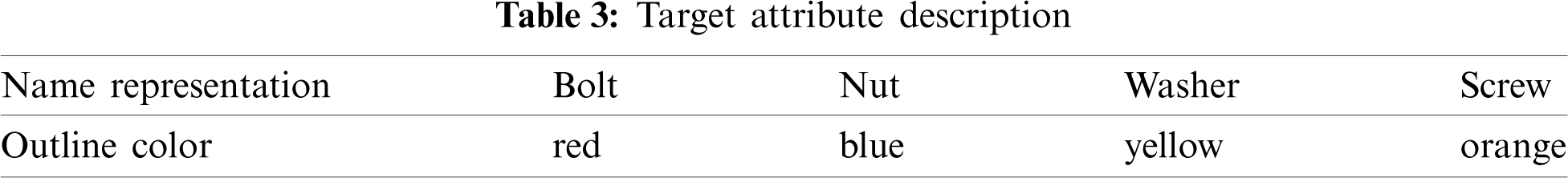
Using YOLOv3-tiny and improved YOLOv3-tiny to detect different bolts, nuts, screws and washers, the description of target attributes is shown in Tab. 3, and the detection effect is shown in Figs. 20 and 21.
YOLOv3-tiny and the improved YOLOv3-tiny algorithm were used to test some images in the test set. The YOLOv3-tiny test results are shown in Fig. 20, and the results of the improved YOLOv3-tiny test are shown in Fig. 21. It can be seen in Figs. 18 and 19 that under the same conditions, the improved YOLOv3-tiny improves the detection accuracy better than YOLOv3-tiny, and some missing frames and small target objects can be framed accurately. This is mainly because the network scale is increased by 52 ∗ 52, and the basic convolutional structure of Mobilev2 has been added to the feature extraction network, which makes the improved network model enhance the detection of small targets, and with the increase of the network layer, the feature extraction capability is improved. A single image tested by YOLOv3-tiny cannot be detected correctly because the parts to be identified overlap. The NMS used in the original YOLOv3-tiny detection framework keeps high reliability frames and deletes frames with low confidence and high overlap, resulting in frame loss. However, the improved YOLOv3-tiny uses the soft NMS algorithm to correctly identify and output frames, thus reducing the frame leakage rate. It can be seen from the test results that the improved YOLOv3-tiny method is more accurate than the YOLOv3-tiny method.
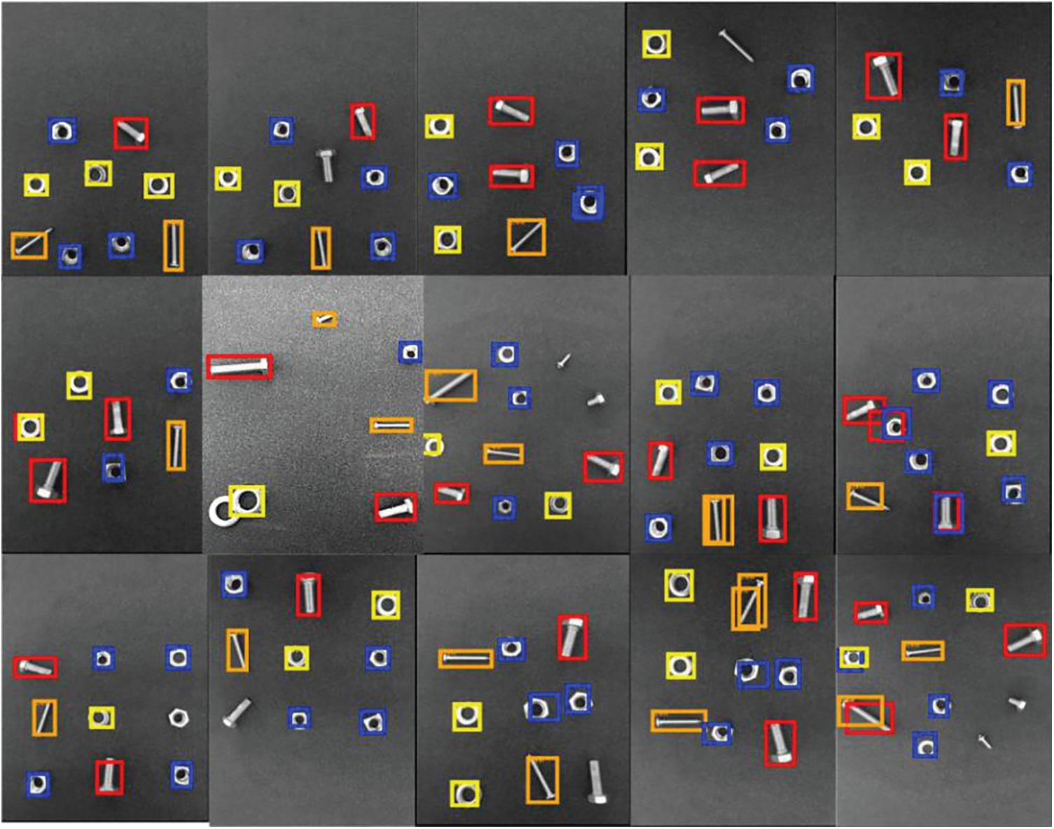
Figure 20: Test effect of YOLOv3-tiny on some test sets
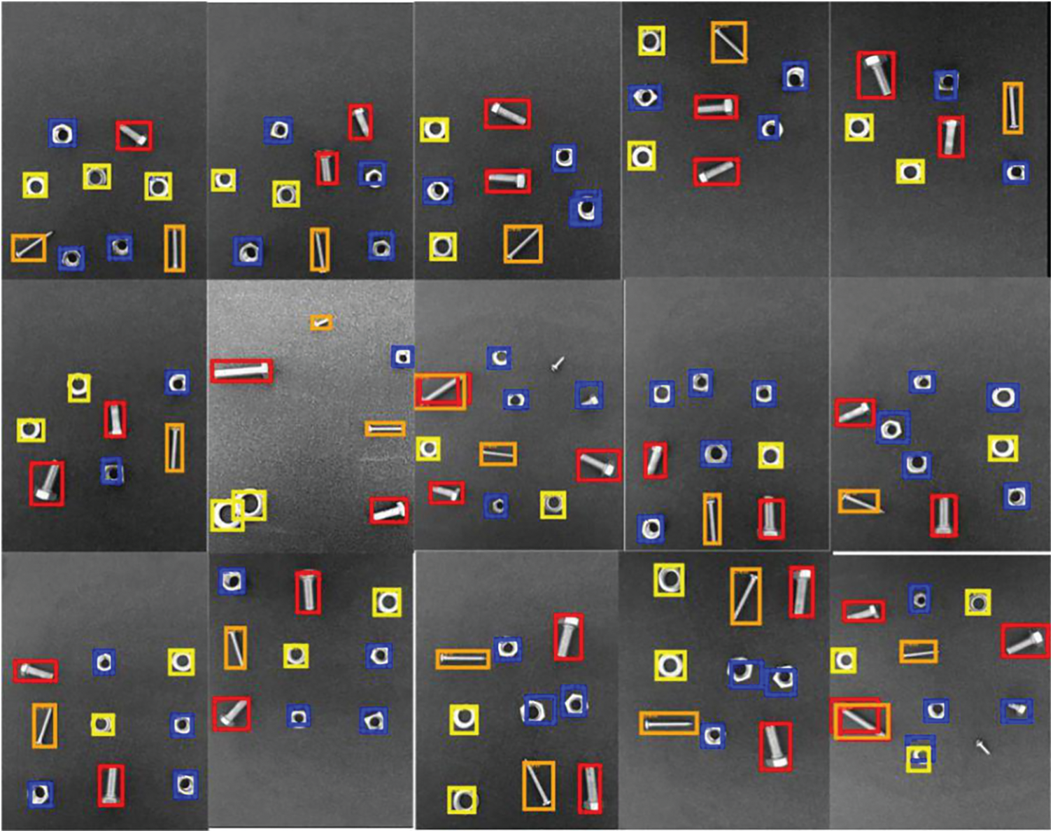
Figure 21: Test effect of YOLOv3-tiny improvement on some test sets
In view of the poor anti-interference ability and low matching accuracy of traditional edge feature matching, an improved target detection algorithm based on YOLOv3-tiny is proposed by using the target detection framework based on deep learning, and the redundant regression frames generated by network prediction are filtered by using the Gaussian weighted attenuation soft NMS algorithm instead of the hard decision NMS algorithm. The network structure not only has a scale of 52 ∗ 52 to improve the detection accuracy of small targets but also uses the basic structure block MobileNetv2 in the feature extraction network, which makes the network perform better.
The experimental results show that in terms of target detection, the improved YOLOv3-tiny target detection algorithm proposed in this paper improves the detection ability of bolts, nuts and screws and improves the accuracy of a single category. The average accuracy rate increases by two percentage points from 0.813 to 0.839, and the recall rate increases by nearly two percentage points from 0.804 to 0.821. In summary, the improved target detection algorithm based on YOLOv3-tiny proposed in this paper has higher accuracy and stronger robustness.
Funding Statement: The authors gratefully acknowledge the support provided by the National Natural Science Foundation of China (No. U20A20265)
Conflicts of Interest: The authors declare that they have no conflicts of interest to report regarding the present study.
1. PR Newswire (2020). Global automotive fasteners industry, vol. 66, no. 2, pp. 368–373, 3117–3120. PR Newswire US. [Google Scholar]
2. Hamdia, K. M., Ghasemi, H., Zhuang, X. Y., Alajlan, N., Rabczuk, T. (2020). Computational machine learning representation for the flexoelectricity effect in truncated pyramid structures. Computers, Materials & Continua, 59(1), 79–87. DOI 10.32604/cmc.2019.05882. [Google Scholar] [CrossRef]
3. Guo, H. W., Zhuang, X. Y., Rabczuk, T. (2019). A deep collocation method for the bending analysis of kirchhoff plate. Computers, Materials & Continua, 59(2), 433–456. DOI 10.32604/cmc.2019.06660. [Google Scholar] [CrossRef]
4. Anitescu, C., Atroshchenko, E., Alajlan, N., Rabczuk, T. (2020). Artificial neural network methods for the solution of second order boundary value problems. Computers, Materials & Continua, 59(1), 345–359. DOI 10.32604/cmc.2019.06641. [Google Scholar] [CrossRef]
5. Wang, Y. B., Hong, K. J., Zou, J., Peng, T., Yang, H. Y. (2020). A CNN-based visual sorting system with cloud-edge computing for flexible manufacturing systems. IEEE Transactions on Industrial Informatics, 7(16). DOI 10.1109/TII.9424. [Google Scholar] [CrossRef]
6. Lowe, D. G. (2020). Distinctive image features from scale-invariant keypoints. International Journal of Computer Vision, 2(60), 91–110. DOI 10.1023/B:VISI.0000029664.99615.94. [Google Scholar] [CrossRef]
7. Ojala, T., Pietikaeinen, M., Maeenpaeae, T. (2002). Multiresolution gray-scale and rotation invariant texture classification with local binary patterns. IEEE Transactions on Pattern Analysis and Machine Intelligence, 7(24), 971–987. DOI 10.1109/TPAMI.2002.1017623. [Google Scholar] [CrossRef]
8. Yang, S., Zhang, J. X., Bo, C. J., Wang, M., Chen, L. J. (2018). Fast vehicle logo detection in complex scenes. Optics & Laser Technology, 110, 196–201. DOI 10.1016/j.optlastec.2018.08.007. [Google Scholar] [CrossRef]
9. Wren, C. R., Azarbayejani, A. (1997). Pfinder: Real-time tracking of the human body. IEEE Transactions on Pattern Analysis and Machine Intelligence, 7(19), 780–785. DOI 10.1109/34.598236. [Google Scholar] [CrossRef]
10. Akcay, S., Kundegorski, M. E., Willcocks, C. G., Breckon, T. P. (2018). Using deep convolutional neural network architectures for object classification and detection within X-ray baggage security imagery. IEEE Transactions on Information Forensics & Security, 9(13), 2203–2215. DOI 10.1109/TIFS.2018.2812196. [Google Scholar] [CrossRef]
11. He, K., Zhang, X., Ren, S., Sun, J. (2016). Deep residual learning for image recognition. Proceedings of the IEEE Computer Society Conference on Computer Vision and Pattern Recognition, pp. 770–778. USA. [Google Scholar]
12. Gkioxari, G., Hariharan, B., Girshick, R., Malik, J. (2014). R-CNNs for pose estimation and action detection. Computer Science, 4(11). [Google Scholar]
13. Girshick, R. (2015). Fast R-CNN. Proceedings of the IEEE International Conference on Computer Vision, pp. 1440–1448. Santiago, Chile. [Google Scholar]
14. Ren, S. Q., He, K. M., Girshick, R., Sun, J. (2017). Faster R-CNN: Towards real-time object detection with region proposal networks. IEEE Transactions on Pattern Analysis and Machine Intelligence, 6(39), 1137–1149. DOI 10.1109/TPAMI.2016.2577031. [Google Scholar] [CrossRef]
15. Redmon, J., Divvala, S., Girshick, R., Farhadi, A. (2017). You only look once: Unified, real-time object detection. IEEE Conference on Computer Vision and Pattern Recognition, pp. 779–788. Washington, USA. [Google Scholar]
16. Liu, W., Anguelov, D., Erhan, D., Szegedy, C., Reed, S. et al. (2016). SSD: Single shot multibox detector. European Conference on Computervision, pp. 21–37. Amsterdam, The Netherlands. [Google Scholar]
17. Redmon, J., Farhadi, A. (2018). YOLOv3: An incremental improvement. Computer Vision and Pattern Recognition, 22, 27–57. [Google Scholar]
18. Zhang, Y., Shen, Y. L., Zhang, J. (2019). An improved tiny-YOLOv3 pedestrian detection algorithm. Optik, 183, 17–23. DOI 10.1016/j.ijleo.2019.02.038. [Google Scholar] [CrossRef]
19. Khokhlov, I., Davydenko, E., Osokin, I., Ryakin, I., Babaev, A. et al. (2020). Tiny-YOLO object detection supplemented with geometrical data. IEEE 91st Vehicular Technology Conference (VTC2020-Spring) Antwerp, Belgium. [Google Scholar]
20. Sun, D. G., Yang, Y., Li, M., Yang, J., Meng, B. et al. (2020). A scale balanced loss for bounding box regression. IEEE Access, 8, 108438–108448. DOI 10.1109/Access.6287639. [Google Scholar] [CrossRef]
21. Bodla, N., Singh, B., Chellappa, R., Davis, L. S. (2017). Soft-nMS-improving object detection with one line of code. Proceedings of the IEEE International Conference on Computer Vision, pp. 5562–5570. Venice, Italy. [Google Scholar]
22. Tsai, R. Y., Lenz, R. K. (1989). A new technique for fully autonomous and efficient 3D robotics hand/eye calibration. IEEE Transactions on Robotics and Automation, 3(5), 345–358. DOI 10.1109/70.34770. [Google Scholar] [CrossRef]
23. Lin, C. H., Lucey, S. (2017). Inverse compositional spatial transformer networks. 30th IEEE Conference on Computer Vision and Pattern Recognition, pp. 2252–2260. Hawaii. [Google Scholar]
24. Zhao, L. Q., Li, S. Y. (2020). Object detection algorithm based on improved YOLOv3. Electronics, 3(9), DOI 10.3390/electronics9030537. [Google Scholar] [CrossRef]
Algorithm Summary
Target Detection Algorithm
In this paper, an improved target detection method based on YOLOv3-tiny is proposed, which adopts the Gaussian weighted attenuation soft NMS (nonmaximum suppression) algorithm, and the MobileNetv2 basic structure block is used in the feature extraction network. The basic concept of the improved YOLOv3-tiny algorithm can be divided into two parts. One is to generate a series of candidate regions in the picture according to certain rules and then mark the candidate regions according to the positional relationship between these candidate regions and the real frame of the object in the picture. An anchor box can be defined by the aspect ratio of the frame and the area (dimension) of the frame, which is equivalent to a series of preset frame generation rules. According to the anchor frame, a series of images may be generated at any position of the image. The calculation formula for the adaptive anchor frame is shown in Eq. (6):
The second part extracts image features by using a convolutional neural network and predicts the position and category of candidate regions. In this way, each predicted frame can be regarded as a sample, and labeled values can be obtained by labeling the real frame with respect to its position and category. The loss function can be established by predicting its position and category through the network model and comparing the predicted value of the network with the marked value. The confidence loss function, the classification loss function and the regression function of the bounding box are expressed in Eqs. (7), (8) and (9):
The calculation of total loss is shown in Eq. (10):
For the Soft-NMS algorithm, first, the NMS algorithm can be expressed by the Eq. (11). bi is the list of initial detection boxes. si contains corresponding detection scores. Nt is the NMS threshold. M is the corresponding box:
To change the hard threshold practice of NMS and follow the principle that the larger the iou, the lower the score (the larger the iou, the more likely it is a false positive), the following formula can be used to express Soft NMS:
However, the above formula is discontinuous, which will lead to faults in the score in the box set, so there is the following Soft NMS formula (which is also used in most experiments):
Eq. (13) assures that when there is no overlap, the continuous penalty function should have no penalty, and when there is a high overlap, it should have a very high penalty.
K-Means Algorithm
The K-means algorithm divides the x matrix of an n sample group into disjunct k clusters. Intuitively speaking, clusters are a collection of data groups, and the data in the cluster are considered to be of the same class. Cluster are the result of clusters. The average of all data in a cluster is usually called the centroid of the cluster. In a two-dimensional plane, the abscissa of the centroid of a cluster of data points is the average value of the abscissa of the cluster data points, and the ordinate of the centroid is the average value of the ordinate. The same principle may also be extended to high-dimensional space.
For a cluster, the smaller the distance between all sample points and the centroid, the more similar the samples in the cluster and the smaller the difference within the cluster. There are many ways to measure distance, and we use absolute distance here. x represents a sample point in a cluster, μ represents the centroid of the cluster, n represents the number of features in each sample point, and i represents the composition of each feature of x. The distance formula from the sample point to the centroid is as follows:
The sum of squares of distances from all sample points to the cluster center is expressed by Eq. (15). m is the number of samples in a cluster, and j is the number of each sample:
 | This work is licensed under a Creative Commons Attribution 4.0 International License, which permits unrestricted use, distribution, and reproduction in any medium, provided the original work is properly cited. |