Computer Modeling in Engineering & Sciences

DOI: 10.32604/cmes.2021.014739

ARTICLE

An Efficient Meshless Method for Hyperbolic Telegraph Equations in (1 + 1) Dimensions

Fuzhang Wang1,2, Enran Hou2,*, Imtiaz Ahmad3, Hijaz Ahmad4 and Yan Gu5

1College of Mathematics and Statistics, Xuzhou University of Technology, Xuzhou, 221018, China
2College of Mathematics, Huaibei Normal University, Huaibei, 235000, China
3Department of Mathematics, University of Swabi, Swabi, 25000, Pakistan
4Department of Basic Sciences, University of Engineering and Technology, Peshawar, 25000, Pakistan
5College of Mathematics, Qingdao University, Qingdao, 266071, China
*Corresponding Author: Enran Hou. Email: houenran@163.com
Received: 26 October 2020; Accepted: 16 April 2021

1  Introduction

The telegraph equation, which has been used to describe phenomena in various fields, belongs to the hyperbolic partial differential equation scope. For example, the telegraph equation in (1 + 1) dimensions can model the vibrations of structures, the digital propagation and also has applications in the other fields [1–3]. Several methods are used to get the analytical/exact solutions of the telegraph equations [4–6]. However, it is almost impossible to get the analytical solutions for relatively complex problems. Thus, numerical approximations to the telegraph equation is a better choice. Some numerical methods have been developed and compared to deal with the hyperbolic telegraph equations [7–9].

Especially, there are several numerical methods concentrate on the second-order 1D linear hyperbolic telegraph equations. For example, Mohanty et al. [10] investigated an unconditionally stable schemes for solving the hyperbolic equations. Based on the finite difference approximation, Dehghan et al. [11–13] presented several methods to simulate the linear hyperbolic telegraph equations. Lakestani et al. [14] used interpolating scaling function technique to solve the 1D hyperbolic telegraph equation. The boundary integral equation accompanied with the dual reciprocity method is used to solve the hyperbolic telegraph equations by Dehghan et al. [15]. Pekmen and Tezer-Sezgin et al. [16] and Jiwari et al. [17] applied the differential quadrature method for the approximate solution of hyperbolic telegraph equations in one-and two space-dimensions. Zerarka et al. [18] considered the 2D generalized differential quadrature method for solving the hyperbolic telegraph equation later. The homotopy analysis method [19] is used to obtain the approximate analytical solution solutions of the second-order 1D linear hyperbolic telegraph equations. A pseudospectral method is proposed by Elgindy [20] for the second-order 1D hyperbolic telegraph equations. The B-spline collocation method is improved by Mittal et al. [21] to get the numerical solutions of the second order 1D hyperbolic telegraph equations. These numerical techniques are based on two-level difference or integral approximations.

Based on the above-mentioned investigations, we propose a direct meshless scheme with one-level approximation for the second-order 1D linear hyperbolic telegraph equations. This is fulfilled by considering time variable as normal space variable. There is no need to remove time-dependent variable during the whole solution process. Under this scheme, we can solve the hyperbolic telegraph equations in a direct way. The rest paper is organized as follows. The formulation of the direct radial basis function is briefly introduced with the methodology for the hyperbolic telegraph equations in Section 2. To cope with the full coefficient matrix derived from the radial basis function method, we propose a simple shifted domain method in Section 3. Section 4 presented some numerical examples to validate the applicability of the proposed direct meshless scheme. Finally, some conclusions are given in Section 5.

2  The Direct Radial Basis Function

The general mathematical formulation of second-order linear hyperbolic telegraph equation in (1 + 1) dimensions is

Lu=∂2u∂t2+2α∂u∂t+β2u−δ∂2u∂x2=f(x,t),0<x<L,t>0 (1)

in terms with the initial condition

u(x,0)=g1(x),ut(x,0)=g2(x), (2)

and boundary conditions

u(x,t)=h(t),t>0. (3)

Here, the coefficient α,β and δ are non-negative constant, f(x,t) is the non-homogeneous/ source term, g1(x),g2(x), and h(t) are prescribed functions. We aim to seek for the solution of unknown function u(x,t).

Almost all numerical techniques for Eqs. (1)–(3) are based on the two-level approximations, most of which are based on the finite difference approximations. Here, we propose a direct collocation scheme by using radial basis function (RBF) under Euclidean space.

2.1 Direct Radial Basis Function

As is known to all, the traditional RBF methods are mostly used to solve 2D or higher dimensional problems. However, there is only one space variable x for Eqs. (1)–(3), we propose a simple direct radial basis function (DRBF) by combining the space variable x and time variable t as a point (x,t) for (1 + 1) dimensional problems. More specifically, the interval [0,L] is evenly divided into segments firstly 0=x0<x1<…<xn=L with corresponding finess h=L/n. The time variable is evenly chosen from the given initial time t0=0 to a prescribed final time tn=T by insert some time points t1,t2,…,tn−1 with time-step Δt=T/n. The corresponding configuration of the space-time coordinate is shown in Fig. 1, where ′∘′ stands for the value of space coordinate/variable x, ′⋅′ represents the value of time coordinate/variable t and ′×′ stands for the point (x,t). Then the DRBF is

ψ(rj)=1+ε2(x−xj)2+ε2(t−tj)2. (4)

The rj=(x−xj)2+(t−tj)2 can be considered as a time-space distance between points (x,t) and (xj,tj). Also, this DRBF is another form of multiquadric radial basis function. One can get the other types of radial basis functions in the DRBF form with little modification.

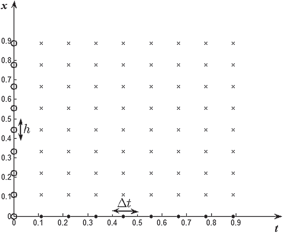
Figure 1: Configuration of the space-time coordinate

Actually, there is another definition of not radial nonmetric space-time radial basis functions with non-geometrical relationship between the space and the time. More details can be found in [22–24].

2.2 Methodology for Hyperbolic Telegraph Equations

According to the definition of DRBF, the above-mentioned Eqs. (1)–(3) can be solved directly in a one level approximation. More specifically, the numerical solution of a function u(x,t) can be obtained from the following approximation

u¯(⋅)≈∑j=1nλjψj(⋅). (5)

We should seek for the unknown coefficients λj(j=1,2,…,n).

The interpolation scheme upon which the Eqs. (1)–(3) collocation is based is as below:

L u¯(xi,ti)=f(xi,ti),(xi,ti)∈(0,1)×(0,T), (6)

u¯(xi,0)=g1(xi),xi∈[0,1], (7)

∂u¯(xi,0)∂t=g2(xi),xi∈[0,1], (8)

u¯(xi,ti)=h(ti),(xi,ti)∈{0,1}×[0,T). (9)

with

Lu¯=∑j=1NλjLψj=∑j=1Nλj(∂2ψj∂t2+2α∂ψj∂t+β2ψj−δ∂2ψj∂x2). (10)

Here, we use NI to denote domain point number, N1 is the point number on boundary t=0 and N2 is the point number on boundary x=0 and x=1 with 2N1+N2=NB denotes the boundary point number. Eqs. (6)–(9) have the matrix form as

Aλ=b, (11)

where A is a N×N known square matrix and b is a N×1 vectors. This can be directly solved by the backslash computation in MATLAB codes.

3  The Shifted Domain Method

It should be noted that for a relatively large physical domain (with large L or T), more collocation numbers are needed to ensure accuracy. For the problems considered in this paper, collocation methods will lead to a full coefficient matrix of linear algebraic equations. This has effect on the numerical solution accuracy. We propose a simple shifted domain method (SDM), which can deal with this problem easily.

The procedure of the SDM is shown by the above-mentioned physical domain Ω1=[0,1]×[0,T), which is also considered as the standard scope. For a larger domain [0,1]×[0,2T) with a larger time 2T, we can first consider the half domain Ω1, the other half domain Ω2=[0,1]×[T,2T) is considered as the shifted domain of Ω1. We can get the numerical solutions on Ω1 and Ω2, respectively. Fig. 2 presents the configuration of the shifted domain in the horizontal direction, where t=T is considered as an artificial boundary. The corresponding solution in the shifted domain Ω2 can be get from the following equations:

Lu¯(xi,ti)=f(xi,ti),(xi,ti)∈(0,1)×(T,2T), (12)

u¯(xi,0)=g1(xi),xi∈[0,1], (13)

∂u¯(xi,0)∂t=g2(xi),xi∈[0,1], (14)

u¯(xi,ti)=h(ti),(xi,ti)∈{0,1}×[T,2T). (15)

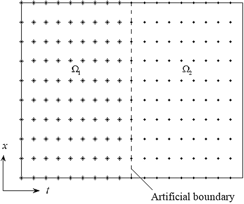
Figure 2: Configuration of the shifted domain in the horizontal direction

This procedure is same as presented in the above-mentioned physical domain Ω1=[0,1]×[0,T). Eqs. (12)–(15), which can be directly solved by the backslash computation in MATLAB codes, have the matrix form as

A˙λ˙=b˙. (16)

where A˙ is a N×N known square matrix and b˙ is a N×1 vectors.

For the other cases, the configuration of the shifted domain in the horizontal direction [0,2]×[0,T) and both directions [0,2]×[0,2T) (with four sub-domains Ω1, Ω2, Ω3, Ω4) are shown in Figs. 3 and 4, respectively.

4  Numerical Experiments

In this section, three examples are considered to validate the DRBF. For fair comparison with the other numerical methods, we use the maximum absolute error (MAE), absolute error and root mean square error (RMSE). The RMSE is defined as [25,26]

RMSE=1Nt−1∑j=1Nt|u(xj,tj)−u¯(xj,tj)|2 (17)

where u(xj,tj) is the analytical solution at test points (xj,tj), j=1,2,…,Nt and u¯(xj,tj) is the numerical solutions at the test points (xj,tj), j=1,2,…,Nt. Nt is the number of test points on the physical domain. Since the parameter ε in the DRBF method is non-sensitive, we fix parameter ε for all the following cases. The optimal choice of DRBF parameter is similar with the other radial basis functions. For more details about this topic, one can be found in [27,28] and references therein.

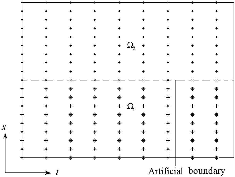
Figure 3: Configuration of the shifted domain in the vertical direction

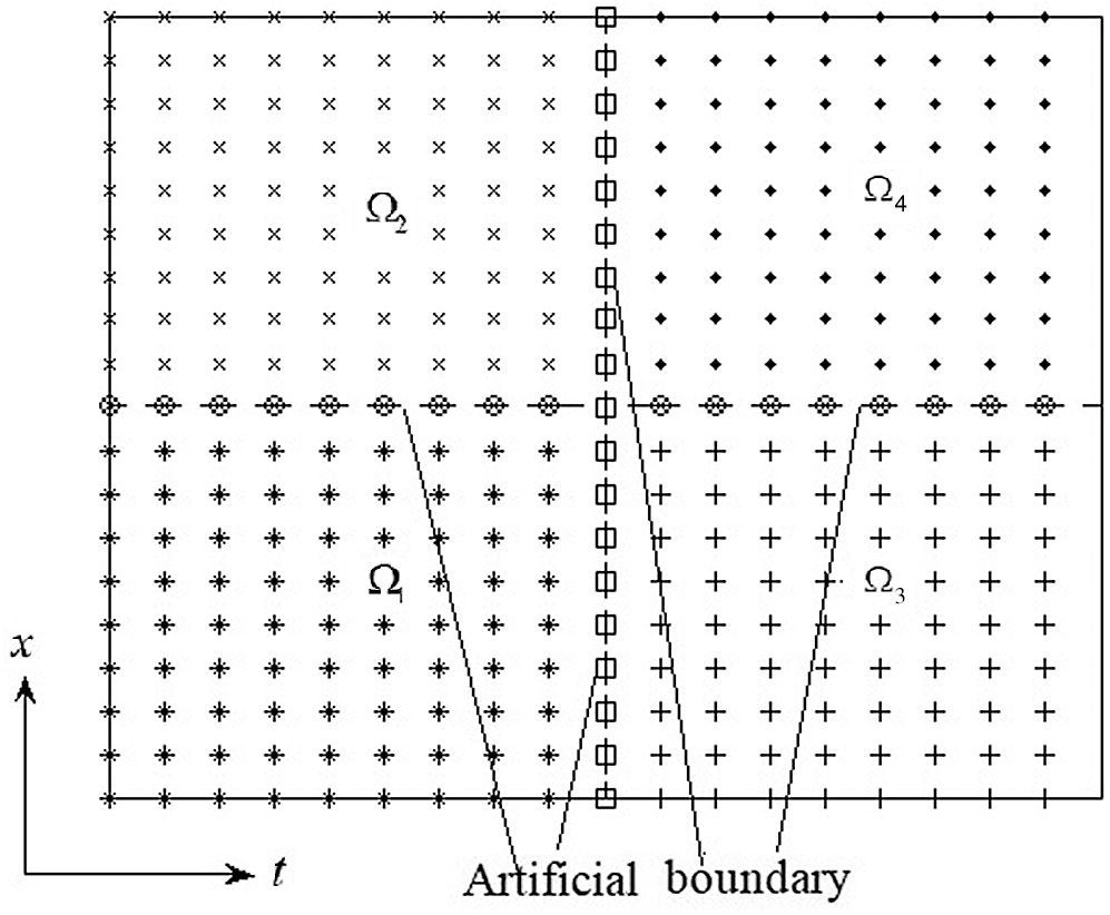
Figure 4: Configuration of the shifted domain in both directions

4.1 Example 1

In order to investigate the DRBF method with the shifted domain method, we consider the hyperbolic telegraph Eq. (1) with the initial conditions

u(x,0)=sin⁡x,0≤x≤π, (18)

ut(x,0)=−sin⁡x,0≤x≤π, (19)

and boundary condition

u(0,t)=u(π,t)=0,0≤t<1. (20)

The corresponding coefficients are α=4, β=2 with analytical/exact solution

u(x,t)=e−tsin⁡x. (21)

The source term is

f(x,t)=(2−2α+β2)e−tsin⁡x. (22)

In this example, the physical domain Ω=[0,π]×[0,1] is divided into three sub-domains, i.e., Ω1=[0,π3]×[0,1] with shifted domains Ω2=[π3,2π3]×[0,1] and Ω3=[2π3,π]×[0,1]. It should be noted that the physical domain division is non-unique. For fixed fineness h=115 and time step △t=115, we compare the DRBF results with the other numerical methods, detailed results with root mean square errors are listed in Tab. 1. We note that our time step △t=115, which leads to less computations, is larger than the one △t=0.0001 in [21,29,30] and △t=0.01 in [15]. Meanwhile, the fineness h=115 is also larger than the reference cases. However, the root mean square errors of DRBF is smaller than the other methods, i.e., the DRBF is more accurate. We note that the DRBF method without the shifted domain method for this case performs not well.

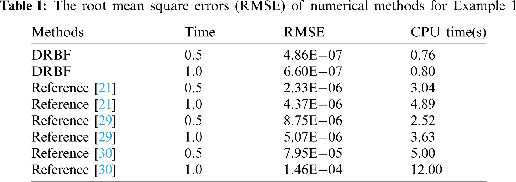
For different mesh sizes H=1/h, Fig. 5 illustrates the root mean square error curve for Example 1 at time T=1. It is seen that the DRBF solutions consistently converge very quickly. The convergence rate is high before reaching the minimum relative error value. It should be noted that the CPU time is 0.27 for mesh size H=1/4 and 1.92 for mesh size H=1/30.

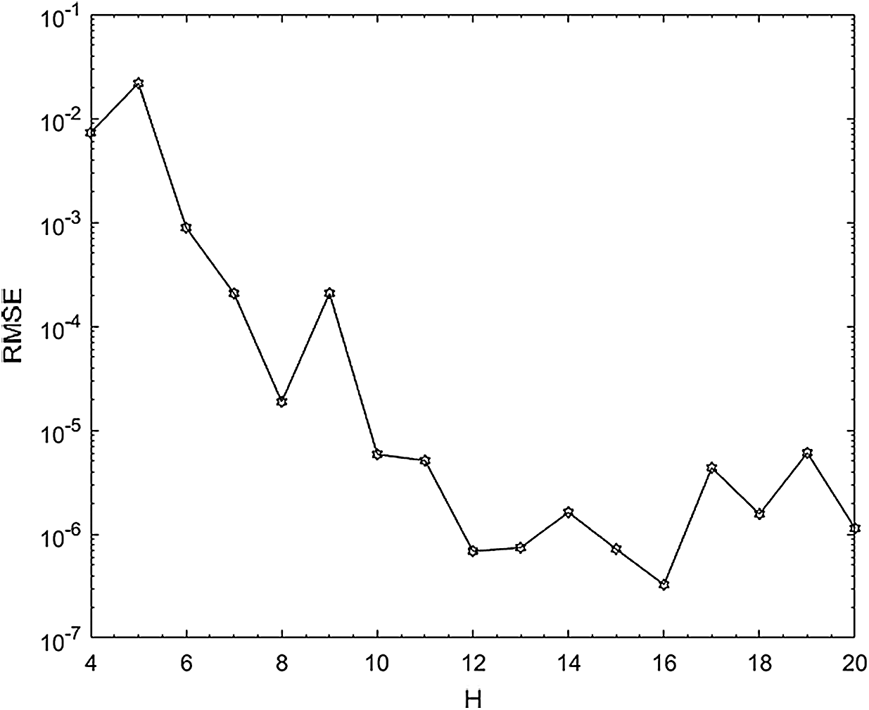
Figure 5: Root mean square error curve for example 1 at time T=1

4.2 Example 2

In order to see the performance of the DRBF with different coefficients, we consider the hyperbolic telegraph Eq. (1) with the corresponding initial conditions

u(x,0)=sin⁡x,0≤x≤π, (23)

ut(x,0)=0,0≤x≤π, (24)

and boundary condition

u(0,t)=0,0≤t≤1, (25)

u(2,t)=sin1cost,0≤t≤1. (26)

The corresponding analytical/exact solution

u(x,t)=sin⁡xcos⁡t. (27)

with source term

f(x,t)=−2αsin⁡xsin⁡t+β2sin⁡xcos⁡t. (28)

For fair comparison with the other methods in [31–33], we consider the maximum absolute errors (MAE) in this example. For space fineness h=115 and time step △t=115, numerical results of the DRBF are listed in Tab. 2 with different coefficients α and β. From which we can find that the DRBF results are stable and accurate for different coefficients. For α=10 and β=5, the solution accuracy of the DRBF is similar with the other methods. For the larger α=20 and β=10, the solution accuracy of the DRBF performs the best.

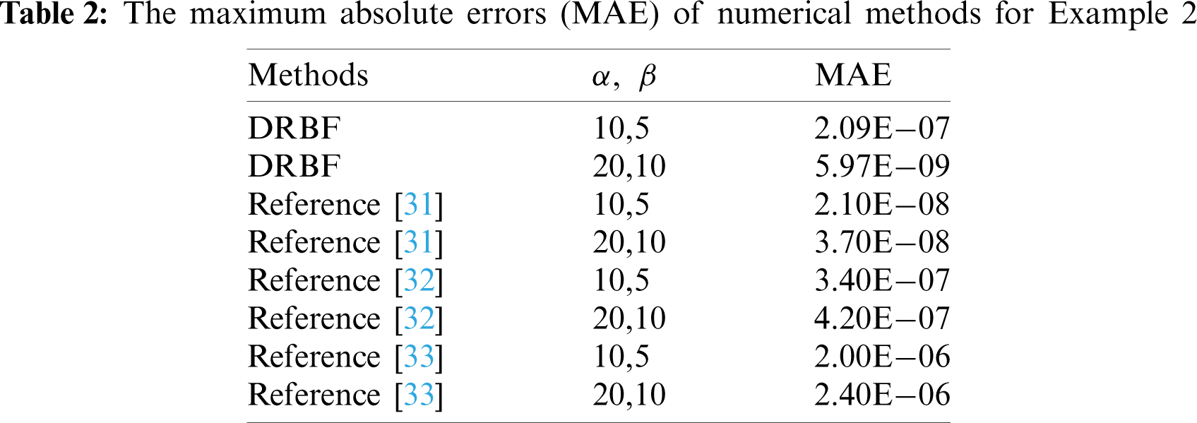
In order to see the difference between the exact and DRBF approximate solutions, Fig. 6 shows the configuration for the larger coefficients α=20 and β=10 at time T=0.5. From which we can see that the numerical solution coincides with the exact solution very well.

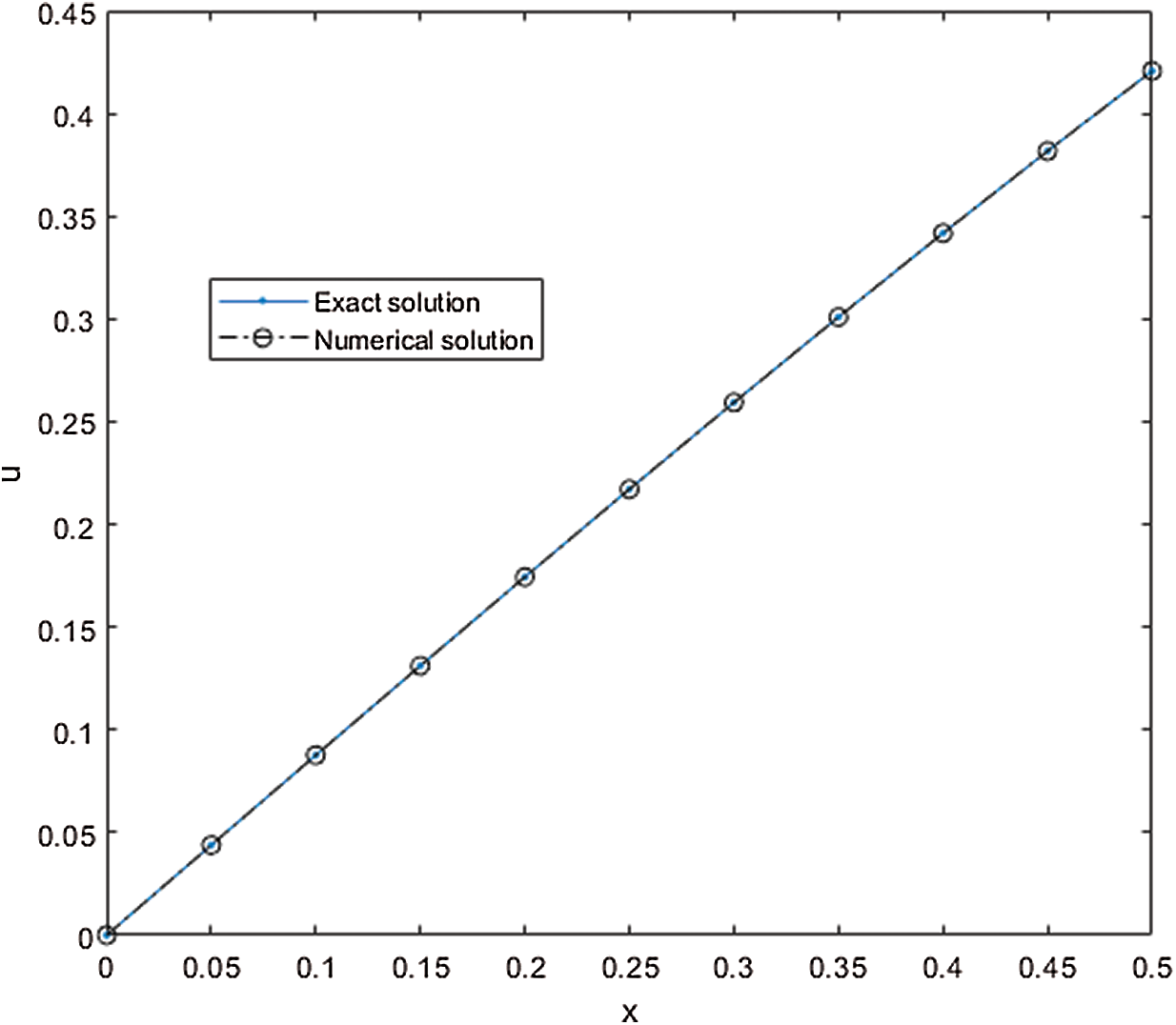
Figure 6: Exact and DRBF approximate solutions for Example 2 at time T=0.5

5  Conclusions

A new direct meshless scheme is presented for the second-order hyperbolic telegraph equations in (1 + 1) dimensions. The present numerical procedure, in which the time variable is considered as normal space variable, is based on the time-dependent radial basis function. There is no need to remove time-dependent variable during the whole solution process. Besides, a simple shifted domain method is proposed to cope with the solution accuracy related to the ill-conditioned coefficient matrix. From the numerical results in Section 4, we find that the proposed meshless method is superior to the other numerical methods. Besides, the direct meshless method can be extended to solve nonlinear problems with Newton iterative method considered. The DRBF with the shifted domain method is promising in dealing with the other types of time-dependent problems, fractional problems [34–36] as well as developing a parallel algorithm for large-scale problems.

Availability of Data and Materials: The data and material used to support the findings of this study are available from the corresponding author upon request.

Funding Statement: The first author is supported by the Natural Science Foundation of Anhui Province (Project No. 1908085QA09) and the University Natural Science Research Project of Anhui Province (Project Nos. KJ2019A0591 & KJ2020B06).

Conflicts of Interest: The authors declare that they have no conflicts of interest to report regarding the present study.

This work is licensed under a Creative Commons Attribution 4.0 International License, which permits unrestricted use, distribution, and reproduction in any medium, provided the original work is properly cited.