Computer Modeling in Engineering & Sciences

DOI: 10.32604/cmes.2021.014107

ARTICLE

MRI Brain Tumor Segmentation Using 3D U-Net with Dense Encoder Blocks and Residual Decoder Blocks

Juhong Tie1,2,*, Hui Peng2 and Jiliu Zhou1,3,*

1College of Computer Science, Sichuan University, Chengdu, 610065, China
2School of Software Engineering, Chengdu University of Information Technology, Chengdu, 610225, China
3School of Computer Science, Chengdu University of Information Technology, Chengdu, 610225, China
*Corresponding Authors: Juhong Tie. Email: tiejuhong@cuit.edu.cn; Jiliu Zhou. Email: zhoujl@scu.edu.cn
Received: 01 September 2020; Accepted: 12 May 2021

1  Introduction

Gliomas are the most widespread malignant brain tumor, accounting for about 70% of primary malignant brain tumors [1,2]. In the light of the World Health Organization (WHO) classification of gliomas, gliomas can be classified into high grade gliomas (HGG) and low grade gliomas (LGG). LGG growth rate is relatively slow and has low malignant degree of tumor and better prognosis of patients. HGG are malignant and more aggressive with faster growth rate and relatively poor prognosis effect. Generally, after diagnosis, the survival time of patients having HGG is about 2 years [3,4]. Therefore, for patients with brain tumor, early detection, diagnosis and treatment is of great value to improve the treatment effect [5,6]. Magnetic resonance imaging (MRI) has developed into the most popular imaging examination for the diagnosis of gliomas in clinical medicine, because it can obtain high-resolution and clear contrast images of brain tissues [7]. According to the degree of invasion, prognosis and other factors, the gliomas show the following sub-regions: peritumoral edema, necrotic core, enhancing tumor core and non-enhancing tumor core [2,3,8]. Multimodal MRI scans are used to reflect the various histological sub-regions by different intensity distribution [9]. The four MRI modalities are T1 weighted (T1), T1 weighted with post-contrast (T1Gd), T2 weighted (T2) and fluid attenuated inversion recovery (FLAIR) [3,5]. Each modality provides different biological information of tumors, which can clearly reflect the internal structure of gliomas. Four MRI modalities axial slices and ground truth segmentation of a patient data (named “BraTS19_TCIA01_201_1”) on the BraTS2019 training dataset is shown in Fig. 1. T2 and FLAIR clearly reflect the whole tumor area, T2 reflects the tumor core and T1Gd reflects the enhancing tumor. Accurate tumor segmentation of MRI modalities is a critical step in clinical diagnosis and efficacy evaluation. Segmentation of MRI brain tumors is difficult, because of the variable location, shape, size and the poorly contrasted boundary with brain normal tissues. Manual segmentation of brain tumors in MR images is time-consuming and is easy to be influenced by the subjective judgment of experts. Therefore, semi-automatic and automatic segmentation of brain tumors have been the important research topics in medical image analysis in recent 20 years, bringing about many kinds of brain tumor segmentation approaches.

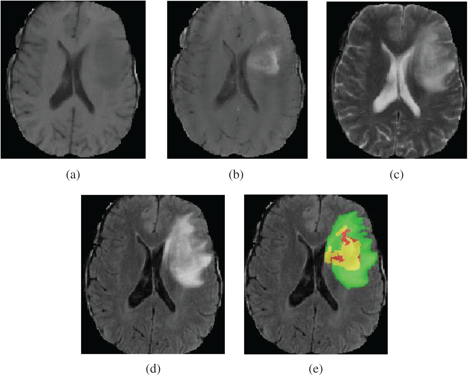
Figure 1: Four MRI modalities axial slices of a patient data from the BraTS2019 training dataset. From (a) to (d) are T1, T1Gd, T2 and FLAIR. (e) The ground truth segmentation, that green indicates edema, yellow indicates enhancing tumor, red indicates non-enhancing tumor and necrotic

According to the existing literature on brain tumor segmentation, the algorithms of brain tumor segmentation can be classified into conventional methods, machine learning approaches (not including deep learning methods) and deep learning methods. Conventional methods mainly include edge detection method [10,11], threshold method [12,13], region growing method [14,15], watershed approach [16,17] and level set approach [18,19]. The conventional segmentation algorithms are fast, low cost, and do not need a powerful computer, but the segmentation result is not good. Machine learning methods use training data to let the machine learn the data features autonomously to achieve object classification and detection. Many researchers [4,20–26] have used machine learning methods to segment brain tumor automatically or semi-automatically and improve the performance of tumor segmentation. The main brain tumor segmentation methods based on machine learning contain support vector machine (SVM) [20,21], clustering based methods [4,22], conditional random field (CRF) [23,24] and random forest method (RF) [25,26]. Bauer et al. [20] combined a classification method based on hierarchial SVM with a CRF-based technique to segment brain tumor of 3D MRI images. Ruan et al. [21] employed Support Vector Machine (SVM) classification to identify the abnormal region and then extract the brain tumor field with multi-scales. Stupp et al. [4] presented Spatially Contrained Fish School Optimization method (SCFSO) and Interval type-II Fuzzy Logic System approaches (IT2FLS) for segmentation of tumor and non-tumor regions in MR brain images. The authors used SCFOS to find out optimal cluster boundaries, and then applied IT2FLS to the next clustering assignment to get the segmentation results. This method achieved good performance with less computing time. Narayanan et al. [22] combined particle swarm optimization (PSO) and bacteria foraging optimization (BFO) with an improved clustering method based on fuzzy c means for segmenting brain tumors in multi modality MR images. Meier et al. [24] used decision forest for classification and conditional random field (CRF) for spatial regularization in brain tumor segmentation. Tustison et al. [25] proposed a supervised brain tumor segmentation method based on random forest (RF) and Markov random field, which yields good segmentation performance for multimodal MRI scans.

In recent years, deep learning which is a particular kind of machine learning has made remarkable achievements in many fields, such as pattern recognition, image segmentation, image detection and image classification [27–29]. Many researchers have applied deep learning methods to automatic MRI brain tumor segmentation. The popular deep learning network architectures are: AlexNet [30], VGGNet [31], InceptionNet [32], XceptionNet [33], U-Net [34], residual network (ResNet) [35] and dense convolutional network (DenseNet) [36]. The early application of deep learning in brain tumor segmentation is mainly to modify the convolution network. Since the U-Net was proposed, it has occupied the main position of brain tumor image segmentation network model because of its good achievements in medical image segmentation [3,37]. Pereira et al. [38] proposed an automatic segmentation method for MRI brain tumors based on 2D CNN. This method predicted the label of the center pixel of a patch, which is time-consuming and does not consider the three-dimensional spatial properties of MR images. With the increasing of GPU memory, many scholars proposed to use 3D CNN to segment brain tumors, and obtained better segmentation results [39,40–42]. U-Net is an architecture which consists of the encoder part and decoder part. The encoder is to capture the context and contain convolution network structure with four times down sampling. The decoder part is to achieve accurate positioning and contain deconvolution network structure with four times upsampling. U-Net has achieved great results in medical image segmentation. Many scholars [37,43–47], have improved the U-Net structure and applied them to MRI brain tumor segmentation, and achieved good segmentation performance. Çiçek et al. [48] proposed a 3D U-Net model based on 2D U-Net. This 3D U-Net can encode more context information and provide dense 3D image segmentation. Mehta et al. [49] revised the original 3D U-Net by taking multimodal MR volumes as input, using multiple scales to process MR volumes, and producing tumor segmentation with multi-labels.

He et al. [35] presented the residual ResNet with the residual block to make the network easier to optimize and solve the degradation problem. ResNet has been broadly applied in image recognition, classification and segmentation. Myronenko et al. [47] added the variational auto-encoder (VAE) branch based on 3D U-Net to regularize the shared encoder, and the original U-Net convolution block was replaced by the residual block. Huang et al. [36] proposed dense convolutional network (DenseNet), in which on the premise of ensuring the maximum information transmission between the layers in the network, all layers were connected directly. DenseNet can alleviate vanishing-gradient, enhance feature propagation, make more effective use of features and reduce the number of parameters. Many researchers have combined DenseNet and U-net for medical image segmentation. MDU-Net [50] is an improved U-net by using three various multi-scale dense connections in encoder, decoder and connection between them. Dense U-net containing 2D dense block both in encoder and decoder was proposed in [51] to segment retinal vessel and achieved a good result. Ziang et al. [52] combined the Inception-Res and dense connection to improve the U-net and yielded perfect performance in medical image segmentation.

Segmentation of brain tumor is very difficult because of the variety of MRI brain tumor images and the small proportion of brain tumor. Although deep learning has achieved remarkable results in MRI brain tumor segmentation, the best results (the first place in the Brats2019 challenge) are: the dice scores of 0.802, 0.909 and 0.865 for enhancing tumor core, tumor core and whole tumor, respectively. Obviously, this segmentation accuracy could not be applied to clinical diagnosis, MRI brain tumor segmentation still has a big room for improvement. Many researchers have proposed plenty of deep neural network models for MRI brain tumor segmentation, but the accuracy problem has not been solved completely. In this paper, we proposed a new network architecture based on U-Net to solve the accuracy problem of MRI brain tumor segmentation.

In our work, by combining the advantages of ResNet and DenseNet, we proposed a new 3D U-Net with residual blocks and dense blocks. Compared with 2D network structure, 3D network model is time-consuming and takes more GPU memory, but it can obtain more feature map information and keep the spatial information of 3D MRI image data, and improve the segmentation accuracy [40,44]. A dense block in DenseNet network is composed of several convolution layers. If the number of input channels of the dense block is K0, the number of its output channels is K0 + K × L. K is the growth rate of the network and L is the number of layers of a dense block. Therefore, the number of output channels of a dense block increases with its layers. This feature of dense block is fit with that of U-Net encoder, because the number of output channels increases with layers in U-Net. And a dense block with fewer parameters obtains better performance than conventional convolution block. Therefore, we applied dense blocks to the contracting path of U-Net encoder. However, in the expanding path, the number of output channels decreases with the network layers. The number of feature maps is decreased and the size of feature maps is increased in the whole decoding process. The dense block has a growth rate factor and the size of feature maps of dense block is growing from input to output, which is not consistent with the characteristics of decoding process. If a 1 × 1 × 1 convolution is added to the output of the dense block to reduce the number of output feature maps, the information will be lost. Therefore, we can not apply dense blocks in the expanding path, but residual blocks. Compared with conventional convolution block, residual block solves the performance degradation problem with the deepening of network layers. Our method is different from the similar methods in [50–52]. In [50] encoder part, the inputs of all the layers before the current layer are linked together, and the encoder of each layer used two traditional 3 × 3 convolutions. The encoder of our work used three layers of dense block, and each layer in the dense block are two 3 × 3 convolutions. The decoder of [50] used two conventional 3 × 3 convolutions, while our work used the residual block. The effectiveness of [51] was not verified in brain tumor segmentation. Wang et al. [51] used 2D dense block in U-net. Our work used 3D dense block in encoder and 3D residual block in decoder. Moreover, the parameters and channel number of dense block in [51] are different from those in our paper. The network structure of [52] is different from our work. In the encoder and decoder part of [52], the first three layers used Inception-Res block, the fourth and fifth layer used Dense-Inception block. The Dense-Inception block is different from dense block in our paper. Each dense layer of the Dense-Inception block used Inception-Res block, while each dense layer of dense block used two traditional convolutions. Our network architecture was trained and validated on the BraTS2019 dataset. The results of experiment demonstrate that our approach has better performance than the original U-Net. And compared with some state-of-art approaches, our approach is a competitive automatic brain tumor segmentation method.

The contributions of this paper are as follows:

(1)   We proposed a new network based U-Net, 3D Dense blocks are used in encoder part and 3D Residual blocks are used in decoder part.

(2)   We presented a new loss function to deal with the case that when all voxels in a patch are non-tumor.

2  Method

2.1 Data and Preprocessing

We used the BraTS2019 dataset, which is divided into training and validation dataset. The BraTS2019 training dataset consists of 335 patients, including 259 HGG and 76 LGG [2,5]. The BraTS2019 validation dataset consists of 125 patients. Each patient includes four modalities: T1, T2, T1Gd, and FLAIR. The size of each modality is 240 × 240 × 155. All modality sequences are co-registered, interpolated and skull-stripped [5]. Each training data is manually annotated by neuroradiologists. There are four kinds of brain tumor segmentation labels: Label 0 for non-tumor area (i.e., background area and normal tissue area), Label 1 for neurotic (NCR) and non-enhancing core (NET), Label 2 for edema (ED) and Label 4 for enhancing tumor core (ET). The regions labeled greater than 0 are called the whole tumor (WT) regions. The regions labeled 1 and 4 are called the tumor core (TC) regions. The regions labeled 4 are called the enhancing tumor (ET) region. The WT regions contain the TC regions, and the TC regions contain the ET region.

Although all MRI images have been pre-processed, the intensities of different MRI images vary greatly. Therefore, we normalized each 3D MR modality image to eliminate the influence of image intensity change on the prediction accuracy. The background voxel value is 0, and brain region voxel value is greater than 0. The normalization is as follows: first, the mean value of the non-zero voxel region is subtracted from the 3D MRI image, and then divided by the standard deviation of the non-zero voxel region.

2.2 Network Architecture

We adopted a U-shaped deep neural network with encoder-decoder. Our network architecture is shown in Fig. 2a. The encoder part obtains the context information of the input image, and the decoder part performs accurate segmentation. The left part of Fig. 2a is the encoder of the network and the right part is the decoder of the network. The encoder is comprised of the input layer, three dense blocks and a residual block. We fed four modalities 3D MR images (T1, T1Gd, T2 and FLAIR) with size 96 × 96 × 96. Thus, the input data is a 4D patch with size 4 × 96 × 96 × 96. The input layer is composed of a 3 × 3 × 3 convolution layer. The input data are four modalities MR images with patch size 4 × 96 × 96 × 96. The number of output channels of the input layer is 16. The dense block consists of three dense layers, and its structure is shown in Fig. 2b. The input of each dense layer is the connection of the output feature maps of all preceding dense layers, which can be expressed as

xi=[y0,y1,…,yi−1](1)

where xi is the input of the ith dense layer, [y0,y1,…,yi−1] is the connecting of the output feature maps of dense layers from 0th to i − 1th, and the output of dense layer 0 is the input of the dense block. The number of output channels of the dense block can be expressed as

kout=kin+kg∗kl(2)

where kout is the number of output channels of the kth dense block. kin is the number of input channels of the kth dense block.kg is the growth rate of the kth dense block, that is, the number of output channels of each dense layer.  kl is the number of dense layers contained in the kth dense blocks. In this paper, kl is 3 and kg is 16, 32 and 64 for the first, second and third dense blocks, respectively.

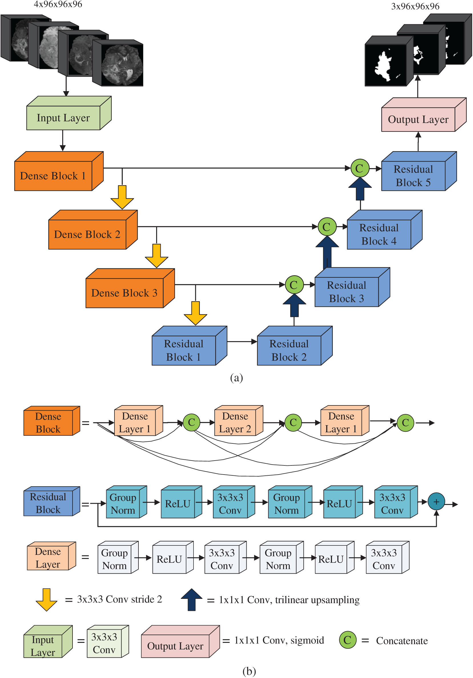
Figure 2: Network architecture

A dense layer consists of one 1 × 1 × 1 convolution layer and one 3 × 3 × 3 × 3 convolution layer. Group normalization and ReLU activation function are used before each convolution layer. When batch size is small, group normalization has better performance than batch normalization [53]. In our work, the batch is 1. Therefore, we used group normalization in the whole network. In a dense block, since each dense layer can access the feature maps of all dense layers before this layer, it gets the global information of the whole block, which is helpful for image segmentation. The growth rate of dense blocks is used to regulate the contribution of the output feature maps of each dense layer to the global information [36].

The structure of the residual block is shown in Fig. 2b, which is comprised of two 3 × 3 × 3 convolution layers. Group normalization and ReLU activation functions are used prior to each convolution layer. The output of the residual block is the addition of the output of the last convolution layer and the input of the residual block. From the top to the bottom of the encoder, the number of feature map increases and the size of feature map reduces progressively. A convolution layer 3 × 3 with step size 2 is used for downsampling to retain more spatial information. The dimension of the output feature map of the bottom layer is 256 × 12 × 12 × 12. Compared with the input, the number of channels increases from 4 to 256, and the size of the feature map is decreased by 8 times.

The decoder of our network is comprised of the output layer and four residual blocks. From the bottom to the top of the decoder, the number of channels decreases and the size of feature maps increases gradually. The decoder performs three upsampling from the bottom to the top by using trilinear interpolation to magnify the feature map. The dimension of the feature map is doubled after each upsampling and it is magnified 8 times in total. The top of the decoder is the output layer consisting of a 1 × 1 × 1 convolution layer and a sigmoid activation function. The feature map size of the output layer is the same as the input image size. The number of the output layer channels is 3. Three feature maps of the output layer are the predicted segmentations of whole tumor, tumor core and enhancing tumor, respectively. In the process of decoding, the input of a decoding block is the concatenation of the upsampled output feature maps of previous decoding block with the output feature maps from the corresponding level of the encoder.

2.3 Loss Function

In the BraTS datasets, approximately 98% of total voxels belong to non-tumor (Label 0, also called background), while only a few voxels belong to tumor (Labels 2, 3, 4). To solve this severe class imbalance, we employed soft dice loss function based regions, as shown in formula (3):

Ldice=13×∑c=13⁡(1−2∑i=1N⁡pci×gci∑i=1N⁡pci2+∑i=1N⁡gci2+ϵ)(3)

where c is tumor region classification, c = 1 for WT, c = 2 for TC and c = 3 for ET. pci is the predicted probability of the ith voxel in class c, 0≤pci≤1.  gci is the groundtruth value of the ith voxel in class c, gci = 1 for the class c and gci = 0 for non-class c. N is the number of total voxels of a patch. To avoid zero division, ϵ is set to 1e-8. If all voxels of a patch only belong to non-tumor region, no matter what the predicted value is, the Ldice calculated by formula (3) is always 1 (gci=0 ∀\,c). Therefore, formula (3) is not suitable for the case where all voxels of a patch are non-tumor. We proposed formula (4) as the loss function.

Ldice=1−1∑i=1N⁡pi2+1(4)

where pi is the predicted probability that the ith voxel belongs to tumor. When the predicted probability of all voxels belonging to tumor is 0, Ldice is 0. On the contrary, when the predicted probability of all voxels belonging to tumor is 1, then Ldice is approximately 1.

2.4 Data Augmentation

Since data in the BraTS2019 dataset are relatively small, we used the data augmentation to prevent over fitting. Our augmentation techniques include random rotation and random flipping. Rotation was performed along the x-axis, y-axis and z-axis with a random probability of 0.15. The rotation angle is −10 to 10 degrees. Flipping was performed along the x-axis, y-axis and z-axis with a random probability of 0.5. In order to save the memory space, we performed these augmentations for each patch during the training process.

2.5 Evaluation Metrics

We used four quantitative evaluations for the segmentation results: Dice Coefficient, Sensitivity, Specificity and Hausdorff Distance [2].

(1)   Dice Coefficient. Dice coefficient is the metric to evaluate the overlap between the manual segmentation and the predicted segmentation. Dice Coefficient can be defined as:

Dice(P,T)=2|T∩⁡P||T|+|P|(5)

where T is the manual tumor segmentation and P is the predicted tumor segmentation.

(2)   Sensitivity. Sensitivity is the proportion of tumor areas that can be predicted correctly. Sensitivity can be expressed as:

Sens(P,T)=2|T∩⁡P||T|(6)

The higher the sensitivity, the higher the proportion of tumor areas predicted correctly.

(3)   Specificity. Specificity is the proportion of non-tumor areas that are correctly predicted. Specificity can be written as:

Spec(P,T)=2|T0∩⁡P0||T0|(7)

where T0 is the manual non-tumor label and P0 is the predicted non-tumor label.

(4)   Hausdorff Distance. Hausdorff distance is the metric to evaluate the distance between manual segmentation boundary and the predicted segmentation boundary. Mathematically, Hausdorff distance is defined as the maximum distance between all points on one set P and the nearest point on another set T, defined as [2]

Haus(P,T)=maxp∈P⁡{mint∈T⁡{d(p,t)}}(8)

where d(p,t) is the Euclidean distance from point p to t. Generally, 95% quantile of Hausdorff distance (i.e., Hausdorff 95) is used as evaluation metric.

3  Experiments, Results and Discussion

3.1 Training

We used Pytorch [54] to implement the network structure, and NVIDIA Geforce GTX1070 GPU with 8 GB memory to train the network. Our network is trained for 260 epochs. The size of a patch is 4 × 96 × 96 × 96. Two patches were randomly selected for each patient in each epoch. Adam optimizer with initial learning rate 1e-4 is employed. The learning rate decreases by 0.75 times per 20 epochs. The L2 regularization of 1e-5 is used to the network weights to prevent overfitting.

3.2 Results and Discussion

BraTS online evaluation tool is employed to measure the performance of the predicted segmentation results. Dice score and Hausdorff distance of prediction segmentation of each patient can be obtained by uploading the prediction results of validation dataset to online evaluation tool. And the average dice score and Hausdorff distance can also be obtained.

Fig. 3a is an example of the training loss curve, which shows the change of training loss with epoch. When epoch is between 0–100, the training loss decreases very quickly. When epoch is 200, the training loss is 0.1146, and epoch is 260, the training loss is 0.1112. Therefore, when epoch is greater than 200, the change of training loss curve is very gentle, which shows the network model is well trained. Fig. 3b shows the training accuracy curve, which is the function of the training accuracy of three regions (WT, TC, ET) varying with epoch. The training accuracy is calculated by soft dice. When the epoch is small, the training accuracy increases faster. When the epoch is greater than 200, three training curves change very gently, this result is expected. It can be seen from Fig. 3b that the training accuracy from high to low is WT, TC and ET. This is because the region area of WT is larger than that of TC, and the region area of TC is larger than that of ET. Therefore, the larger the tumor area is, the higher the training accuracy is.

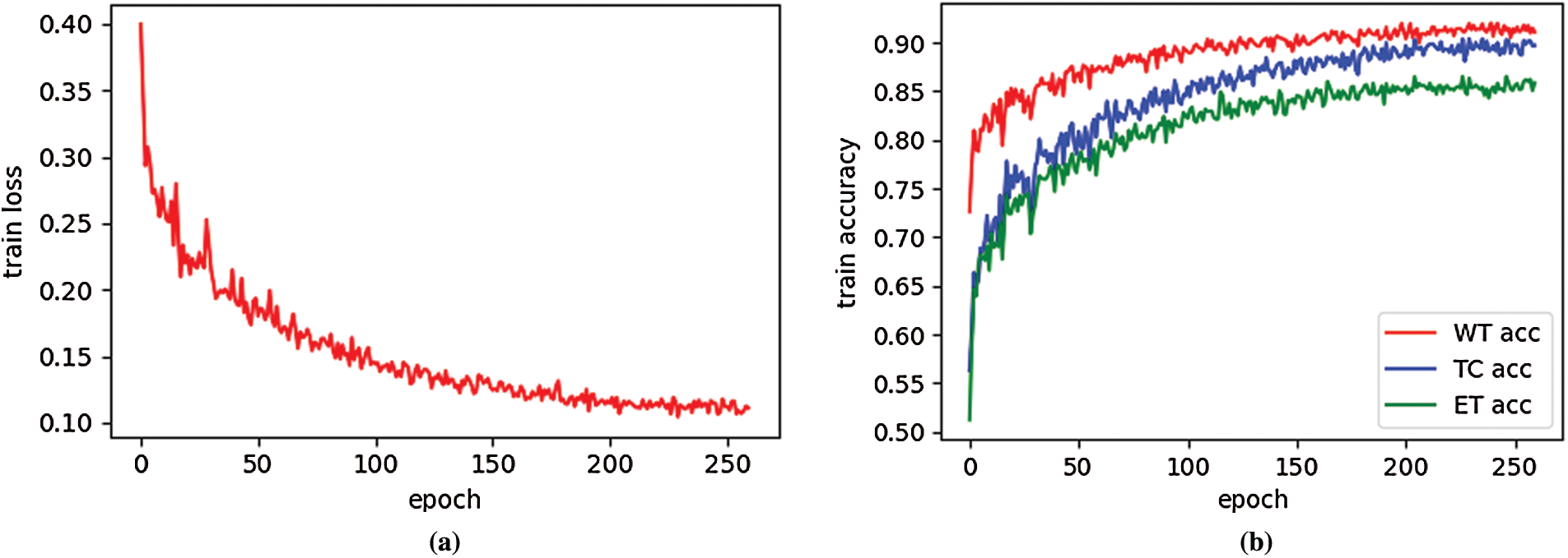
Figure 3: Training loss curve (a) and train accuracy curve (b) on BraTS2019 training dataset

Fig. 4 shows boxplots of dice score, sensitivity, specificity and hausdorff95 obtained by our network on BraTS2019 validation dataset. The boxplots reflect the divergence of these metrics. As can be seen from Fig. 4a, the dice score of WT region has the minimum divergence and the maximum mean. Fig. 4b shows that the sensitivity of WT region has the minimum divergence and the maximum mean value. The specificity of the ET region has the minimum divergence and the maximum mean, as shown in Fig. 4c. Hausdorff95 of ET region has the minimum divergence and the minimum mean value, as pictured in Fig. 4d.

Figure 4: Boxplots for each of the three tumor sub-regions on the BraTS2019 validation set. (a) the boxplots of dice score; (b) the boxplots of sensitivity; (c) the boxplots of specificity; (d) the boxplots of 95% quantile of the Hausdorff distance. The mean is denoted using a red ‘X’

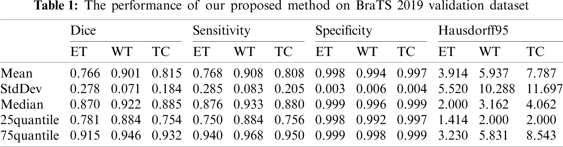
Our segmentation results were obtained on BraTS2019 validation dataset, and the performance indicators are shown in Tab. 1 which lists the value of dice, sensitivity, specificity and Hausdorff95 of ET, WT and TC in the three regions. The average value, standard deviation, median value, 25% quantile value and 75% quantile value are given for each indicator value. It can be seen from Tab. 1 that the dice of WT, TC and ET are 0.901, 0.815, and 0.766, respectively, and the Hausdorff95 of ET, WT and TC are 3.914, 5.937 and 7.781, respectively. In our method, the highest prediction accuracy is WT region, and the lowest is ET region. This is because WT region is the largest, and ET region is the smallest. The larger the region is, the easier it is to be predicted. And the smaller the region is, the harder it is to be predicted.

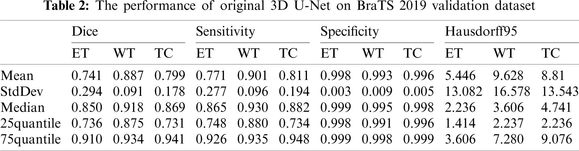
The performance of our method is compared with the original 3D U-Net method. The main difference between original 3D U-Net network and our network is the encoding block and the decoding block. In this paper, the encoding and decoding block structure of original 3D U-Net is: Groupnorm -> Relu -> 3 × 3 × 3 conv -> Groupnorm -> Relu -> 3 × 3 × 3 conv. Except for the different network, the training process, training data and training parameters are the same. The original 3D U-Net segmentation results obtained on the Brats2019 validation dataset are shown in Tab. 2. For mean metris in Tab. 2, we found that the dice of WT, TC and ET are 0.887, 0.799 and 0.741, respectively, and the Hausdorff95 of ET, WT and TC are 5.446, 9.628 and 8.81, respectively. Comparing the data in Tabs. 1 and 2, the dice of WT, TC and ET obtained by our method are higher 0.014, 0.016 and 0.025 than original 3D U-Net, and the Hausdorff95 of ET, WT and TC are lower 1.532, 3.691 and 1.029 than original 3D U-Net. The Sensitivity of WT and the Specificity of WT and TC of our method are also higher than original 3D U-Net. Four segmentation evaluation metrics of WT of our method are all better than the original 3D U-Net. The values of Sensitivity-ET and Sensitivity-TC of the original 3D U-Net are better than our method. Specificity-ET of our method and the original 3D U-Net is the same. We also noted that all median metrics excluding Sensitivity-TC by our method are better than the original 3D U-Net. Our method has superior overall performance to the original 3D U-Net. There are two reasons why our method is better than the original 3D U-Net. First, we used dense block in the encoder, while original 3D U-Net used traditional convolution block. Compared to traditional convolution block, dense block has the advantages of deepening network layers, strengthening feature propagation, avoiding gradient vanishing, and expanding the receptive field. Second, residual block was used in our network decoder, while traditional convolution block was used in original 3D U-Net. The shortcut connection of residual block improves the efficiency of information flow, and so solves the degradation problem.

Our method was qualitatively compared with original 3D U-Net. We randomly selected a patient and used both our method and original 3D U-Net to segment the brain tumor. Fig. 5 shows slices of the four modalities, the ground truth of the patient named “BraTS19_2013_21_1,” and the slices of the predicted segmentation image using our method and original 3D U-Net.

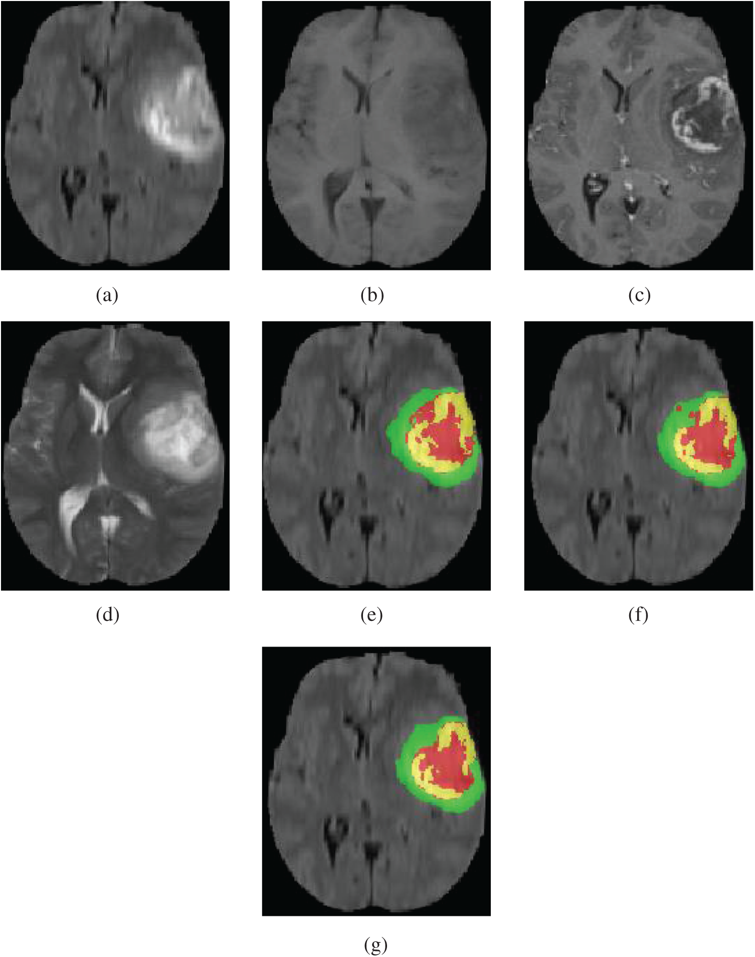
Figure 5: Four modalities axial slices, ground truth and segmentation results of a patient from Brats2019 training dataset using our network and original 3D U-Net. Yellow indicates enhancing tumor core, green indicates edema, red indicates necrotic and non-enhancing tumor core in (e), (f) and (g). (a) FLAIR, (b) T1, (c) T1Gd, (d) T2, (e) Ground truth, (f) original 3D U-Net, (g) our network

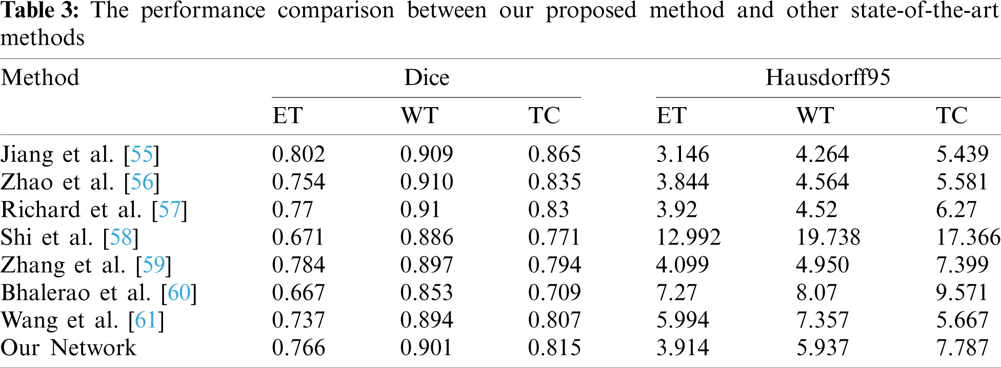
Tab. 3 shows that the performance comparison of our method with some the most advanced methods. Jiang et al. [55], won the first place in the BraTS2019 challenge, proposed a two-stage cased U-Net and used two branches decoder in the second stage U-Net. Their Dice and Hausdorff95 metrics are better than our method. The Dice-ET of [55] and our method are 0.802 and 0.766, respectively, and the difference is small. Zhao et al. [56], ranked the second place, studied different kinds of methods of 3D brain tumor segmentation and combined them to improve the segmentation accuracy. The value of Dice-ET of our method is 0.766, and higher 0.012 than [56]. The other values of Dice and Hausdorff95 in [56] are better than our method. Modified DeepSCAN model with instance normalization and local attention was proposed by McKinley et al. [57] who won the third place in BraTS 2019 challenge. Their overall performance is better than our method. But the Hausdorff95-ET of our method is 3.914, better than the third place, and the Dice-ET between two methods is very close. Shi et al. [58] presented a dense channels 2D U-Net, and used residual block and feature pyramid structure. Our method performance especially in Hausdorff95 metrics is superior to [58]. Zhang et al. [59] extended 3D U-Net by using dense connections, and used LeakyReLU and 3D batch normalization. They also used postprocessing by replacing ET when its voxels number is less than 300 with non-enhancing and necrotic tumor methods to improve Dice-ET value, and obtained the excellent Dice-ET which is higher than our method. The other metrics value of our method are all higher than achieved by Zhang et al. [59]. Bhalerao et al. [60] extended the original 3D U-Net using residual connections in both encoder and decoder part. They also use postprcessing method the same as in [59], but the threshold of ET voxels number is obtained by mean-dice, rather than setting a fixed value like in [59]. But their extensions and postprocessing method for enhancing ET Dice did not get good results. Wang et al. [61] used 3D U-Net with the residual connections in encoder unit, and applied two different patches in training and prediction. Their performance metrics excluding Hausdorff95-TC are not better than our method. From above analysis, we can conclude that our method achieved a good performance on ET region. This is because the ET region is very small and it is very hard to predict. If a patient has no ET tumor and a voxel is predicted as ET tumor, then the dice of BraTS evaluation is zero. Our loss function learns this situation and improves ET prediction accuracy. Compared with these state-of-the-art methods, our proposed method achieves some competitive performance. The main reason why our method has better performance than those methods [58–61] is that our method has superior network architecture which used dense blocks and residual blocks to improve prediction accuracy of segmentation. One of the reasons why our method is worse than those methods [55–57] is that our patch size is only 96 × 96 × 96 due to GPU memory limitations. The patch size of those methods [55–57] is larger than 96 × 96 × 96, and the larger patch contains more contextual information which are beneficial to achieve high dice scores [55].

4  Conclusion

In the training process, we used only 8 G memory of the GPU. Because of the limitation of GPU memory, the dimension of the patch in the experiment is relatively small (4 × 96 × 96 × 96). According to the existing research reports, the larger the patch size is, the better the segmentation performance is. We believe that when the patch size is larger, the performance of our method will be better.

According to the characteristics of MRI brain tumor segmentation, combined the advantages of DenseNet and ResNet, this paper proposed a deep 3D full connected convolution network similar to U-Net with encoder-decoder. Dense block is used in encoder and residual block is used in decoder. In encoding process, with the increase of layers, the number of output feature maps increases, which is consistent with the characteristic of dense block. The advantage of using dense block is to reduce network parameters, deepen network layers, strengthen feature propagation, avoid vanishing-gradient problem, and enlarge the receptive fields. Compared with traditional convolution block, residual block solves the problem of network performance degradation with the increase of network depth. The soft dice loss function shown in formula (3) is not suitable for the case where all voxels of a patch belong to the non-tumor. Therefore, we proposed a loss function as shown in formula (4), which forces the network to increase the segmentation accuracy of a patch that all voxels are non-tumor.

We obtained the dice of WT, TC and ET are 0.901, 0.815 and 0.766 respectively on the BraTS2019 validation set, which is better than the original 3D U-Net. Compared with some state-of-the-art methods, our method is also a competitive automatic brain tumor segmentation method. The application of this method in clinical oncology can help radiologists and oncologists to get various tumor regions, sizes and shapes, and assist them in improving tumor diagnosis, treatment plan and prognosis.

Funding Statement: This was supported partially by Sichuan Science and Technology Program under Grants 2019YJ0356, 21ZDYF2484, 21GJHZ0061, and Scientific Research Foundation of Education Department of Sichuan Province under Grant 18ZB0117.

Conflicts of Interest: The authors declare that they have no conflicts of interest to report regarding the present study.

This work is licensed under a Creative Commons Attribution 4.0 International License, which permits unrestricted use, distribution, and reproduction in any medium, provided the original work is properly cited.