Computer Modeling in Engineering & Sciences

DOI: 10.32604/cmes.2021.015922

ARTICLE

Forecasting Model of Photovoltaic Power Based on KPCA-MCS-DCNN

Huizhi Gou1,2,* and Yuncai Ning1

1School of Management, China University of Mining and Technology-Beijing, Beijing, 100083, China
2China Energy Investment Corporation, Beijing, 100011, China
*Corresponding Author: Huizhi Gou. Email: ghz_0262@163.com
Received: 24 January 2021; Accepted: 21 April 2021

Abbreviations

1  Introduction

With the world's energy crisis becoming increasingly serious and the environmental pollution caused by the burning of fossil fuels intensifying, the development of clean and renewable energy has become the consensus of the entire human race [1]. Among them, the conversion and utilization of solar energy, with its advantages of less restricted environmental conditions and low equipment maintenance costs, has received widespread attention and been vigorously promoted in many countries. The use of photovoltaic power generation has undoubtedly had a significant alleviating effect on the current dual crisis of energy and environment [2].

Photovoltaic power is affected by real-time weather and diurnal alternation, and is significantly volatile, random and intermittent. Fluctuations in the total amount of PV power on the grid will have a significant impact on the safety and stability of the power system, as well as on the scheduling of the power system, the marketing of power and the bidding of the power generation companies for the grid [3]. Therefore, accurate PV power forecasting is of great value and significance.

In terms of PV power prediction, there have been related studies at home and abroad, in which the prediction methods are mainly divided into two categories: physical methods and statistical methods [4]. The approach of the physical method, which addresses the logical relationship between meteorological data and PV power, investigates the key influencing factors of PV power based on physical principles. With regard to this approach, existing studies often adopt satellite cloud maps to obtain data on the movement, coordinates and size of the clouds in the sky, which leads to predictions of the variability of ground irradiance and ultimately to PV power predictions [5]. The physical method does not require a large amount of historical data and is suitable for new PV plants, but requires detailed geographical information of the PV plant and data such as module parameters. It has a complex modeling process. It is also difficult to simulate some extreme abnormal weather conditions and slow changes in the environment and PV module parameters over time. In summary, the model is poorly resistant to disturbances and not very robust [6].

Statistical methods refer to the employment of historical data to find the intrinsic laws between data changes and data relationships, and thus to accomplish forecasting [7]. For example, the time series methods represented by autoregressive moving average model (ARMA), autoregressive integrated moving average model (ARIMA), autoregressive model with exogenous input (ARX) and autoregressive moving average model with exogenous inputs model (ARMAX) [8] are mainly applicable to the situation where the weather conditions are more stable, while this method does not have high prediction accuracy due to the simpler conditions. Classification regression methods represented by support vector machines (SVM) and decision trees classify PV power into specific classes and situations based on the idea of clustering to filter similar days closer to the target in a smaller range [9]. Neural network algorithms represented by back propagation neural network (BPNN) and wavelet neural network have been widely applied in research in recent years with the rapid development of artificial intelligence [10]. In addition, random forest algorithms exist, i.e., decision trees based on data sampling are built and interlinked to achieve a PV power prediction model capable of filtering noise and fluctuations [11]. Another approach is the probabilistic prediction algorithm, which gives the probability distribution of the PV power taken at a certain time period [12]. From this, it can be found that the statistical model part of the existing research mainly uses shallow learning algorithms such as SVM and BPNN, which can only learn the information contained in the data from lower dimensions and cannot fully reflect the characteristics of the information, so it is necessary to introduce deep learning algorithms into PV power prediction research.

The true computational power of neural networks came into play in 2006 when Professor Hinton of the University of Toronto pioneered the “multi-layer structure, layer-by-layer learning” deep neural network [13]. The pioneering of deep neural networks has attracted a great deal of attention from academia and industry, and with in-depth research and development of deep learning, it has become a popular tool in the field of data analysis in the era of big data [14]. This approach has made breakthroughs in areas such as signal recognition and natural language processing, and continues to set various records within various application areas at an astonishing rate. Deep convolutional neural networks were proposed by Krizhevsky et al. in 2012 by introducing the concept of deep learning on top of the traditional convolutional neural networks (CNN) [15]. This network is widely applied because it can effectively avoid complex data processing and can learn data features autonomously. In fact, DCNN is the first learning algorithm that can successfully train a multilayer network [16]. The DCNN model achieves optimization of the neural network structure by autonomously feeling convolution, weight sharing, subsampling and multiple perceptual layers for local features [17]. The DCNN model not only reduces the number of neurons and weights but also makes the input features displacement, scaling and warping invariant using the pooling operation, thus improving the accuracy and robustness of network training [18].

Although DCNN has shown good prediction performance, it still suffers from the problem of blind parameter selection and therefore needs to be optimized by choosing a suitable intelligent algorithm [19]. The cuckoo search algorithm (CS) is an emerging heuristic algorithm proposed by Professor Xinshe Yang and S. Deb of Cambridge University in 2009 [20]. Compared with particle swarm algorithm and genetic algorithm, this algorithm has a relatively high performance for solving optimization problems. It is inspired by the cuckoo's parasitic hatchling breeding method to solve optimization problems. The algorithm is favored by many research scholars for its simple structure and few control parameters, and has become a current research hotspot [21]. However, in the process of optimization, it was found that the CS algorithm has disadvantages such as the tendency to fall into local optimality [22]. In order to overcome the shortcomings of the CS algorithm and improve the accuracy and efficiency of the optimization, this paper introduces the concept of random weights for improvement, and employs random weights to change the update method of the bird's nest position in order to improve convergence speed of the algorithm and achieve the global optimal search.

Furthermore, there are many factors affecting PV power that are coupled with each other, and if all the influencing factors are used as input indicators for the prediction model, there will be a large amount of redundant data, so feature selection is also important [23]. Principal component analysis (PCA), as a multivariate statistical method that combines multiple variables into a small number of variables [24], is better at dealing with individual indicators that have a strong linear relationship. However, the relationship between the factors affecting PV power is often non-linear. In contrast, principal component analysis is a linear method that cannot obtain higher-order features of the data and ignores the non-linear information of the data while reducing the dimensionality [25]. Therefore, in this paper, kernel principal component analysis is adopted to reduce the dimensionality of the input variables while retaining the non-linear information among the input variables by mapping the initial input variables to a high-dimensional feature space through a non-linear transformation.

To sum up, this paper constructs a PV power prediction model based on a modified CS algorithm to optimize DCNN, and applies KPCA to reduce PV power influencing factors. The remainder of the article is organized as follows. The second part introduces the algorithms used in paper, which include KPCA, modified cuckoo search algorithm and DCNN model. The third section constructs a complete framework for PV power prediction. The accuracy and robustness of the proposed models are tested and analyzed in the fourth section using practical examples. The fifth section summarizes the research results of paper.

2  Basic Theory

2.1 Kernel Principal Component Analysis

PCA, as a multivariate statistical method that combines multiple variables into a few, has a good treatment when dealing with individual indicators that have a strong linear relationship [26]. However, the relationship between the factors affecting PV power is often non-linear. And principal component analysis is a linear method that cannot obtain the higher-order characteristics of the data and ignores the non-linear information of the data while reducing dimensionality. Therefore, this paper utilizes KPCA to extract key factors, which can effectively deal with the non-linear relationship between variables and is widely employed in the comprehensive analysis of multiple indicators, and can achieve more reasonable results than PCA.

Kernel principal component analysis is a non-linear principal component model that maps the initial input variables to a high-dimensional feature space through a non-linear transformation, reducing the dimensionality of the input variables while retaining the non-linear information between them, in order to accurately extract the important information features between the variables to obtain the main input indicators. This methodology can compress information contained in a large number of indicator variables into a small number of composite variable indicators that reflect the original information characteristics, and deal with the non-linear relationships between variables through the analysis of the composite variable indicators, while ensuring that the loss of information in the original data is minimized. The underlying steps are as follows [27].

Set a group of random vectors X={x1,x2,…,xn}T containing variables, where xk∈RN(k=1,2,…,m) and m represents the number of input samples. The original input sample data set is M=[a1,a2,…,an]T=[b1,b2,…,bm]. The projection of data set into the space F through the nonlinear mapping Φ is M=[φ(b1),φ(b2),…,φ(bm)], satisfying ∑k=1mφ~(bi)=0.

The covariance matrix is obtained as follows:

CF=[C11,C12,…,C1n…Cn1,Cn2…,Cnn](1)

C=1m∑imφ(bi)φ(bi)T(2)

The eigenvalue and eigenvector can be obtained as follows:

CFWF=λFWF(3)

where λF is the eigenvalue and WF=∑k=1Mαkφ~(xk) is the eigenvector corresponding to the eigenvalue. Define a symmetric matrix K whose elements are:

K(xk,xj)=(φ(xk)⋅φ(xj))(4)

K~ can be obtained by matrix centralization:

K~=K−InK−KIn+InKIn(5)

where In is n×n matrix, Iij=1/n, and Eq. (3) can be simplified as:

mλFM=K~M(6)

As a result, the kernel principal component can be calculated by referring to extraction technique of traditional PCA.

2.2 Modified Cuckoo Search Algorithm

Cuckoo search algorithm is a novel heuristic algorithm proposed by Professor Xinshen Yang and S. DEB of Cambridge University in 2009 [28]. The CS algorithm outperforms particle swarm optimization (PSO) and genetic algorithm (GA) in solving optimization problems mainly owing to its fewer parameters, simplicity of operation, ease of implementation, excellent stochastic search paths, and strong merit-seeking capability. Its outperformance is mainly manifested in better convergence and stronger robustness. It is inspired by the breeding method of cuckoo parasitizing and brooding. Currently, cuckoo search algorithm has been widely applied in project scheduling, engineering optimization and other fields. Due to its simple structure and few control parameters, this algorithm is favored by many researchers and has become a research hotspot.

2.2.1 Cuckoo Search Algorithm

The core idea of CS is the breeding pattern of cuckoo and Levy flight [29].

(1)   Breeding pattern of cuckoo

According to the long-term observation and research of entomologists, cuckoos do not raise their offspring, but secretly put their nestling birds in the nests of other birds. If they are not found by the owner of the nest, the offspring will be raised. All along, cuckoo does not build nests or hatch young eggs. It will search for birds which have similar shapes and sizes of eggs. These birds also have similar breeding period and similar feeding habits. Cuckoo will watch other birds. When they leave the nest, cuckoo will quickly lay eggs in Orioles, skylarks and other birds’ nests, and let them hatch on their own behalf. Because the color and size of the eggs are very similar, cuckoo will remove one egg from its original nest before laying eggs, and at the same time they give birth to one of its own, so that its young can enjoy the care of other birds. The cuckoo's characteristic is to find a nest, parasitize and incubate. CS is a simulation of this behavior. The core idea is to regard the nest selected by cuckoo as the distribution of solution in space, and whether the nest location is good or not symbolizes the fitness value of the solution to the problem. The series of proceedings of the cuckoo searching and deciding on a nest represents the whole process of optimization performed by the algorithm.

(2)   Levy flight

CS adopts Levy flight search method, which satisfies random distribution of heavy tail. The walking step length is short distance and long distance, which will show up alternately. Employing Levy flight mode can increase search space, expand population diversity and jump out of local optimum. Several important parameters in Levy distribution are characteristic index α, scale σ, displacement χ and direction parameter β. The definition of Levy distribution is the Fourier transform of its characteristic function.

pα,β(k;μ,σ)=F{pα,β(x;μ,σ)}=∫−∞∞dxeikxpα,β(x;μ,σ) = exp⁡[iuk−σα|k|α(1−iβk|k|ϖ(k,α))](7)

where ϖ(k,α)={tan⁡πα2,α≠1,0≺α≺2−2πln⁡|k|,α=1

The probability density function of Levy flight distribution is shown below:

pα,β(x)={12πx−23exp⁡(−12x),x≥00,x≺0,(8)

where α = 12, β = 1.

The jump distribution probability density function of Levy flight is presented in the following formula:

λ(x)≈|x|−1−α,0≺ε≺2(9)

Since Levy flight is a function of second-order divergence, its jumping in motion is very large.

2.2.2 Modification of Cuckoo Search Algorithm

CS has been successfully applied to the field of nonlinear optimization, and has obtained good optimization results. It has excellent local and global convergence, and it needs fewer parameters. Consequently, it has a strong robustness and high search efficiency. However, in the process of optimization, it has been found that Cuckoo search algorithm emerges with some drawbacks such as slow convergence speed and long operation time [30]. In order to overcome the shortcomings of CS and improve the accuracy and efficiency of optimization, the concept of random weight is introduced to improve CS. The random weight is adopted to change the update mode of bird's nest position. The ultimate goal of these measures is to improve the convergence speed of the algorithm and realize the global optimal search.

Random weight is a dynamic approach to select weights from Gaussian distribution. This method can avoid CS falling into local optimum in the initial stage of search, and the random appearance of large and small weights can also improve the slow convergence speed and low precision of the algorithm in the later stage.

w=0.5+randm()2(10)

where randm() represents a random number and obeys normal distribution. According to the literature [31], the formula is to generate a value randomly between [0.5,1].

w=rmin+(rmax−rmin)∗normrnd()+σ∗randm()(11)

where rmax and rmin represent the maximum and minimum values of randomly selected weights, respectively. normrnd() represents a random number and obeys uniform distribution. σ represents deviation.

The random weight obeys Gaussian distribution, w∼N(θ,σ). Due to the random appearance of large and small weights, the algorithm can find the optimal solution more easily and get the balance of local and global search. Using the random weight can change the updating mode of the nest position, hence this paper proposes a cuckoo optimization algorithm based on random weight. The specific flow is as follows:

Step 1: Determine the optimization function f(x), set the objective function dimension d, definition domain [−l,l], discovery probability P0 (the probability of new nest replacing old nest) and population number n. Initialize the population n and generate d-dimensional vector (x1,x2,⋯,xn)T randomly. The initial position of n nests is Si(i=1,2,⋯,n).

Step 2: Calculate objective function fi of each nest and record the current optimal solution. The reciprocal of mean absolute percentage error is defined as the objective function.

Step 3: Keep the optimal position of the previous nest Sit, generate weights w∼N(θ,σ) randomly, replace the position of the previous generation with a new position and update it. The formula is as follows:

Si(t+1)=w∗Sit+α⊕Levy(λ)(12)

where t represents the number of iterations, α is the step size, and ⊕ is the point-to-point multiplication. This formula represents a random walking equation. The first term of the current equation and the second term of the transition probability equation determine the position of the next generation. Levy flight is a random search path whose step size satisfies Levy distribution.

Step 4: Compare the updated nest position Sit + 1 with the previous position Sit. If the current position is better than the previous position, in other words fit+1 \gt fit, Sit + 1is regarded as the current optimal position, otherwise, the previous position Sit remains unchanged.

Step 5: Compare the random number of the possibility of the nest owner to discover the eggs of foreign birds compared with the probability of discovery (the parameter value has been determined in the parameter setting). If r≤P0, the current position will be recorded as the optimal position; otherwise, it will be turned to Step 2, and the position of the nest will be changed randomly to get a new set of positions for comparison.

Step 6: Output the global optimal solution which satisfies the above conditions, including fit+1 \gt fit and r≤P0.

2.3 Deep Convolutional Neural Network

A deep convolutional neural network is an artificial neural network with deep learning capability, mainly characterized by locally connected and shared weights of neurons in the same layer. Convolutional neural networks are generally composed of multiple feature extraction layers and a fully connected layer at the end, with each feature extraction layer consisting of a convolutional layer and a sub-sampling layer. The neuron nodes between layers in deep convolutional neural networks are no longer in the form of full connectivity, but rather the neuron nodes of each adjacent layer are linked to only the upper layer neuron nodes that are close to it exploiting the layer space correlation. In other words, local connectivity is achieved, which greatly reduces the parameter size of the network [32]. The structure of DCNN is displayed in Fig. 1.

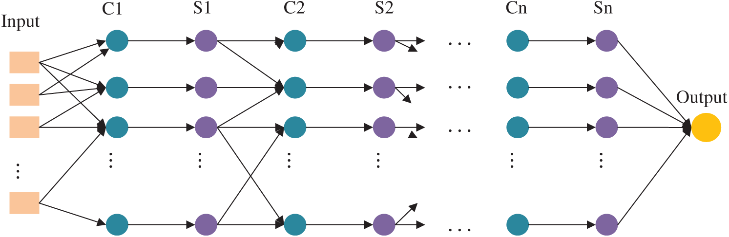
Figure 1: The typical DCNN structure

A classic DCNN structure mainly consists of the input layer, the convolutional layer, the subsampling layer and the fully connected layer. The convolutional layer is mainly utilized for feature extraction through convolutional kernels to achieve feature vector extraction and enhancement [33]. In the convolutional layer, the output features of the previous layer are convolved with the convolutional kernel for a convolutional operation, and the feature output of this convolutional layer is calculated by weighting the activation function, as shown in the following equation:

xjl=f(∑j=mkxjl−1wjl+θjl),j=1,2,…,n;0<m≤k≤n(13)

where f(I)=11+e−I,I=∑j=mkxjl−1wjl+θjl(j=1,2,…,n;0<m≤k≤n), xjl is the value of corresponding position on the output dataset of the first layer; xjl - 1 is the value of corresponding position on the input dataset of layer l−1; j takes the value of m to k to denote that it is a local connection; wjl is the weight value of convolution kernel; and θjl is the threshold value.

The subsampling layer is mainly employed to subsample the features of the convolutional layer by performing a “pool averaging” or “pool maximization” operation [34] for each sample pool of n×n size in the subsampling layer to extract sample features as follows:

xjl=g(xjl−1)+θjl(14)

where xjl, xjl−1 and θjl represent the same meaning as Eq. (13); g represents the function that selects the average or highest value. By pooling operations, the complexity of convolution layer is effectively reduced, the overfitting phenomenon is avoided, and the fault tolerance of the feature vector to microdeformations of data features is improved, enhancing the computational performance and robustness of the algorithm.

The data obtained after the above convolutional and subsampling layers will eventually be connected to the fully connected layer [35]. The fully connected layer is formulated as follows:

xl=f(Il),Il=Wlxl−1+θl(15)

where f(∼) and θl represent the same meaning as in Eq. (14), Wl is the weight value when l calculating the layer to l−1 layer, and xl is the output data.

In the aforementioned calculation process, each convolutional kernel is repeatedly applied to all the input data by sliding, and multiple sets of output data are obtained by convolving several different convolutional kernels, with the same convolutional kernel having the same weight, and the output data of different sets are combined and then output to the sub-sampling layer. The sub-sampling layer takes the output data of the previous convolutional layer as input data, first sets the range of value locations, then fills the range with the average or maximum value of the range by sliding, and finally combines these data to obtain the reduced dimensional data and outputs the result through the fully connected layer [36].

The application of DCNN for PV power prediction has two major advantages: firstly, it allows for the existence of malformed data; secondly, it reduces the number of some parameters through local connectivity and weight sharing, which improves the efficiency and accuracy of PV power prediction. However, the number of parameters that need to be trained in the prediction application needs to be determined subjectively, which affects the stability of the prediction results. To further improve the operational efficiency and prediction accuracy, this paper will adopt the MCS algorithm to optimize the parameters of DCNN.

3  Implementation of PV Power Prediction Model

Based on the aforementioned theory, the KPCA-MCS-DCNN prediction model is constructed in this paper. Fig. 2 illustrates the flow of PV power prediction based on KPCA-MCS-DCNN.

As depicted in Fig. 2, the model firstly performs feature dimensionality reduction on the impact factor of PV power by KPCA method, then applies MCS to optimize the parameters of DCNN, and finally employs DCNN to train the sample set to obtain the optimal prediction model. The detailed procedures are as follows:

(1)   Select initial input variables (xi) and process data. By analyzing the PV power characteristics, generate the initial set of input variables X={xi,i = 1,2,… n}, and standardize data of each input factor (xi).

(2)   Extract features via KPCA. After Step (1), the original input variable matrix X is generated, and the Gaussian kernel function is selected for the non-linear mapping function. After the non-linear transformation of Eqs. (1) to (6), the kernel principal components are extracted according to the criterion that the cumulative variance contribution rate τ is higher than 95%, and the new input variable matrix is finally formed.

(3)   Initialize parameters. Initialize the weights w and thresholds θ in DCNN by randomly selecting a number of values from a smaller set of values as the weights and all thresholds for each layer.

(4)   Optimize DCNN with MCS. If the conditions are met, the optimal parameters are obtained; if the conditions are not met, the MCS optimization algorithm is executed again until the set of solutions that meet the conditions is obtained.

(5)   Simulation prediction. The prediction model obtained from the above optimization training is employed to predict PV power, and the proposed model is compared with MCS-DCNN, CS-DCNN, DCNN and BPNN. Furthermore, the results are analyzed and evaluated by adopting root mean square error (RMSE), mean absolute percentage error (MAPE) and mean absolute error (MAE). These three indicators are calculated as follows [37]:

RMSE=(1N)∑t=1N(yt−yt∗)2(16)

MAPE=1N∑t=1N|yt−yt∗yt|×100(17)

MAE=(1N)∑i=1N|yt−yt∗|(18)

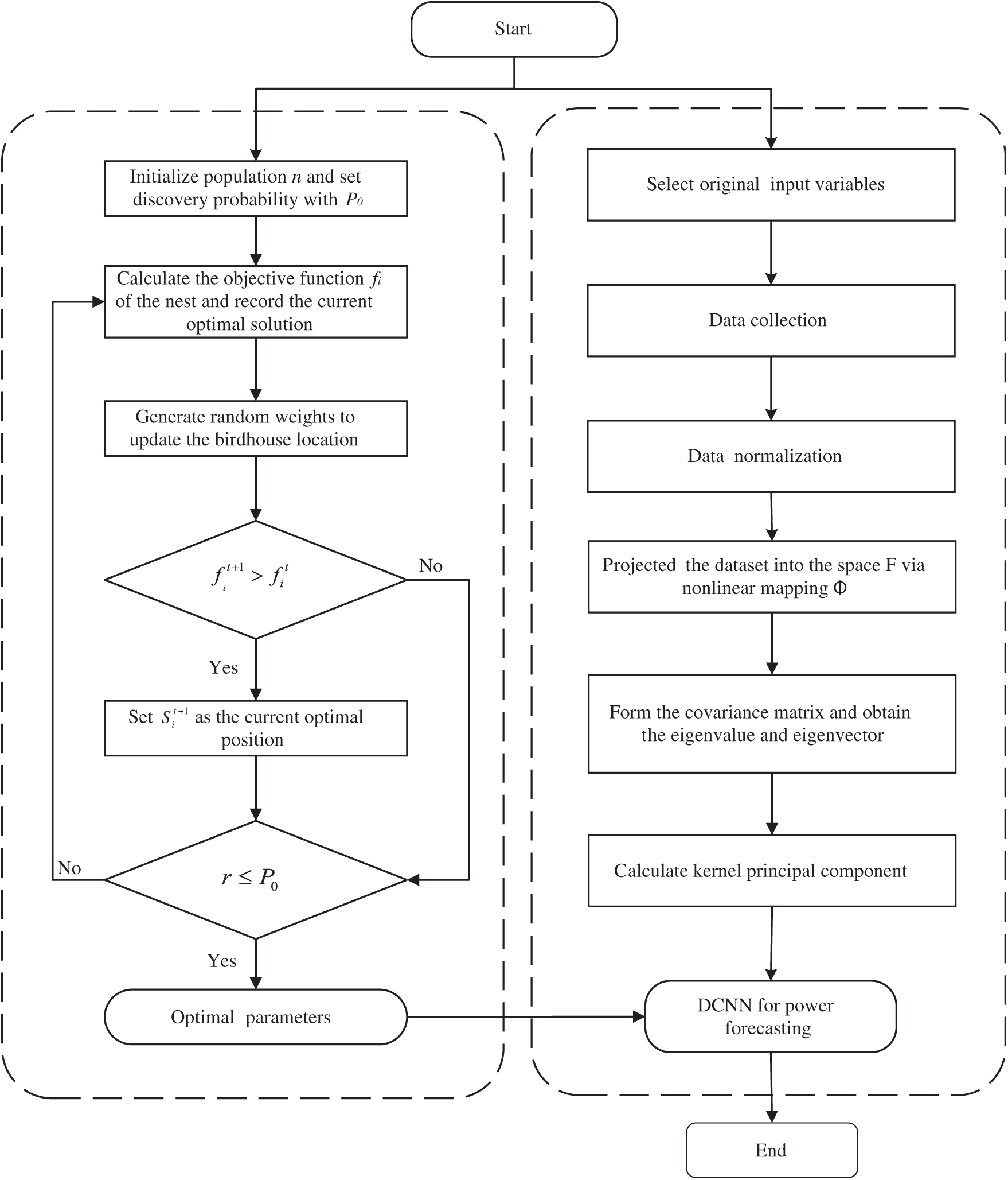
Figure 2: Prediction flow based on KPCA and DCNN optimized by MCS

where yt is the actual PV power value, yt∗ is the predicted PV power value and N is the number of data sets. The smaller the value of the above indicators, the higher the prediction accuracy.

4  Case Study

4.1 KPCA Analysis

The data used for the calculations in this section is from a PV farm in China. In this paper, weather data and PV power data are selected as the initial input features for the model. In particular, weather data contains 12 independent variables: total precipitation, cloud ice content, surface air pressure, relative humidity, total cloud cover, horizontal wind speed, vertical wind speed, atmospheric temperature, surface solar radiation, ground thermal radiation, extra-atmospheric solar radiation and sediment amount. In addition to these factors, the PV power data at T-i (i = 1, 2, 3, 4, 5, 6) time points are also selected as the initial input features.

The variance contribution and cumulative contribution of the 18 indicators are illustrated in Tab. 1. In order to more visually observe and compare the calculated results of PCA and KPCA, Figs. 3 and 4 are plotted.

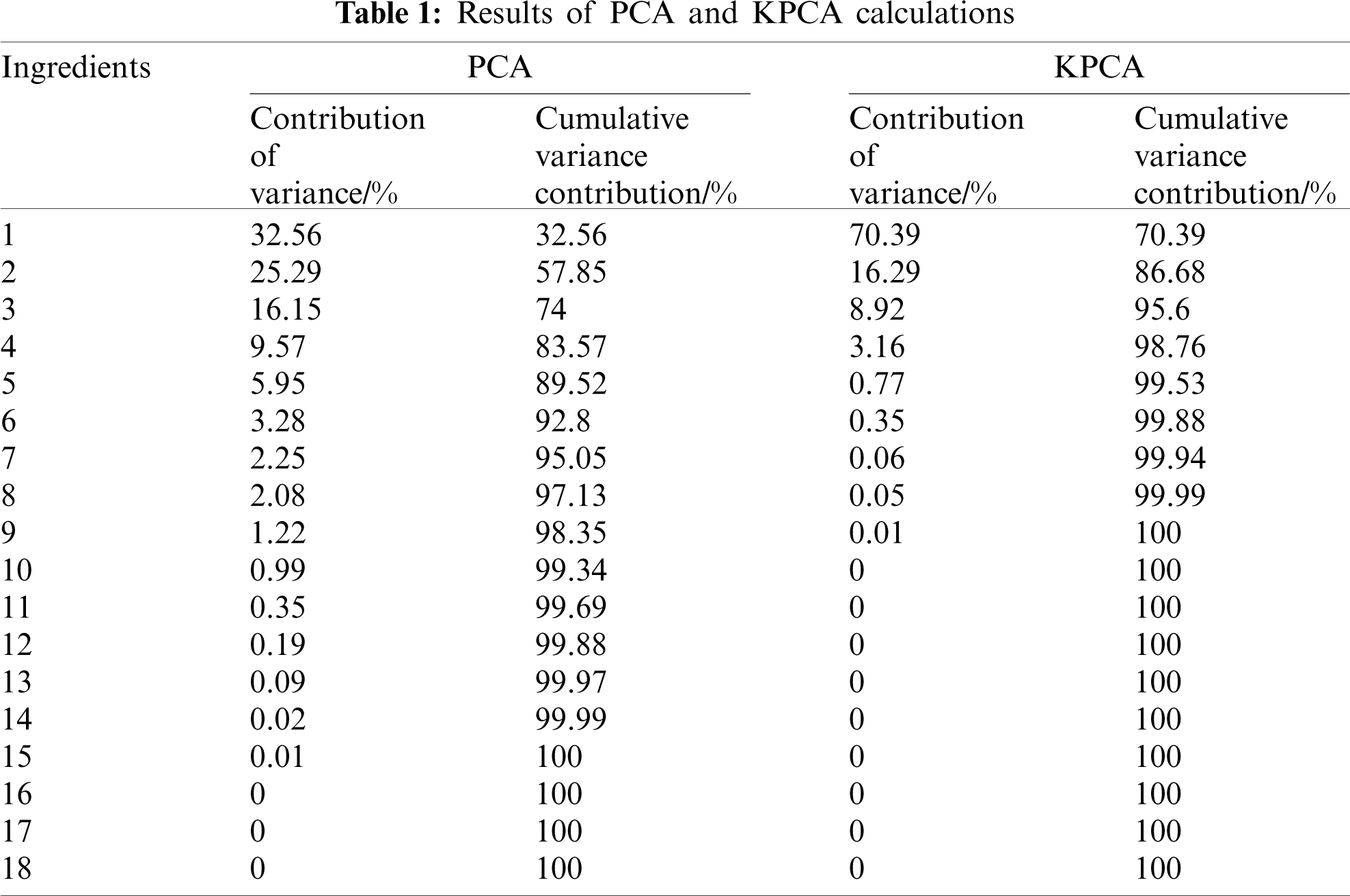
As can be seen from Tab. 1 and Figs. 3 and 4, the contribution rate of the first principal component of KPCA reached 70.39%, covering 70.39% of information of original data. After the principal component analysis of each indicator, the contribution rate of the first principal component was obtained to be lower, only 32.56%, which was much smaller than the contribution rate of the first principal component of KPCA. What's more, if the cumulative contribution rate exceeds 95%, PCA requires the extraction of 7 principal components, which is closer to the original number of indicators than KPCA, which only requires the extraction of 3 principal components. It can be concluded that KPCA is significantly stronger than PCA in terms of dimensionality reduction and problem simplification, and the extracted principal components retain sufficient information of the original data.

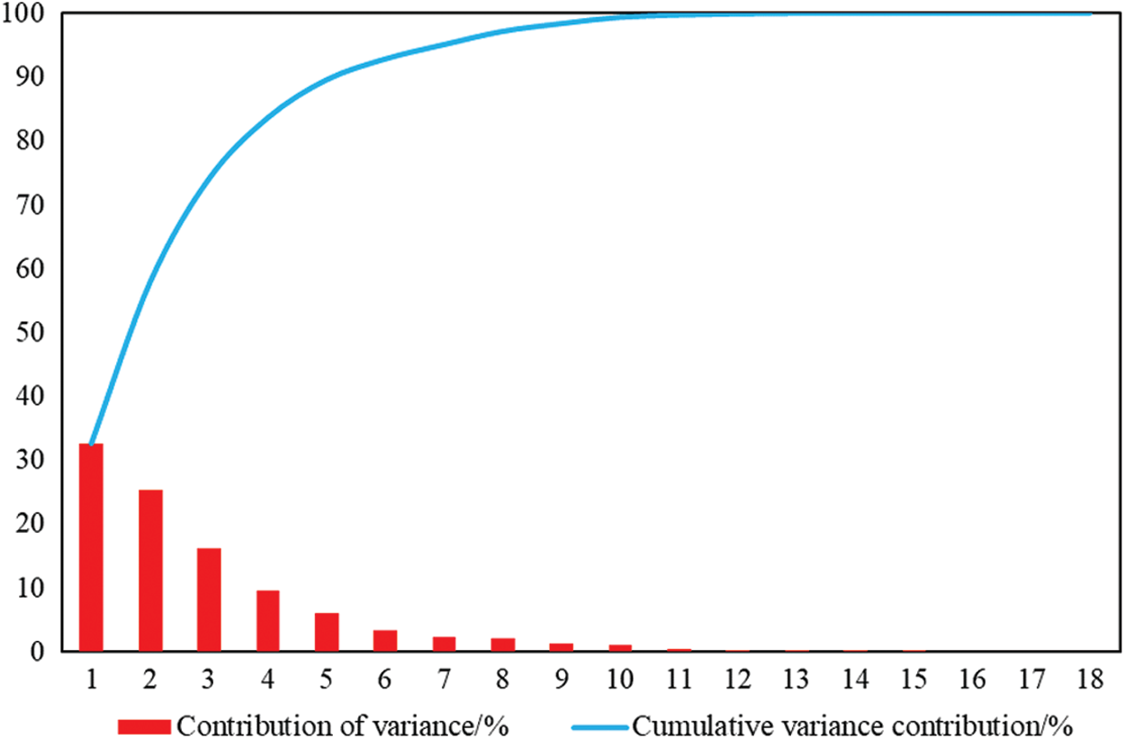
Figure 3: Total variance of PCA

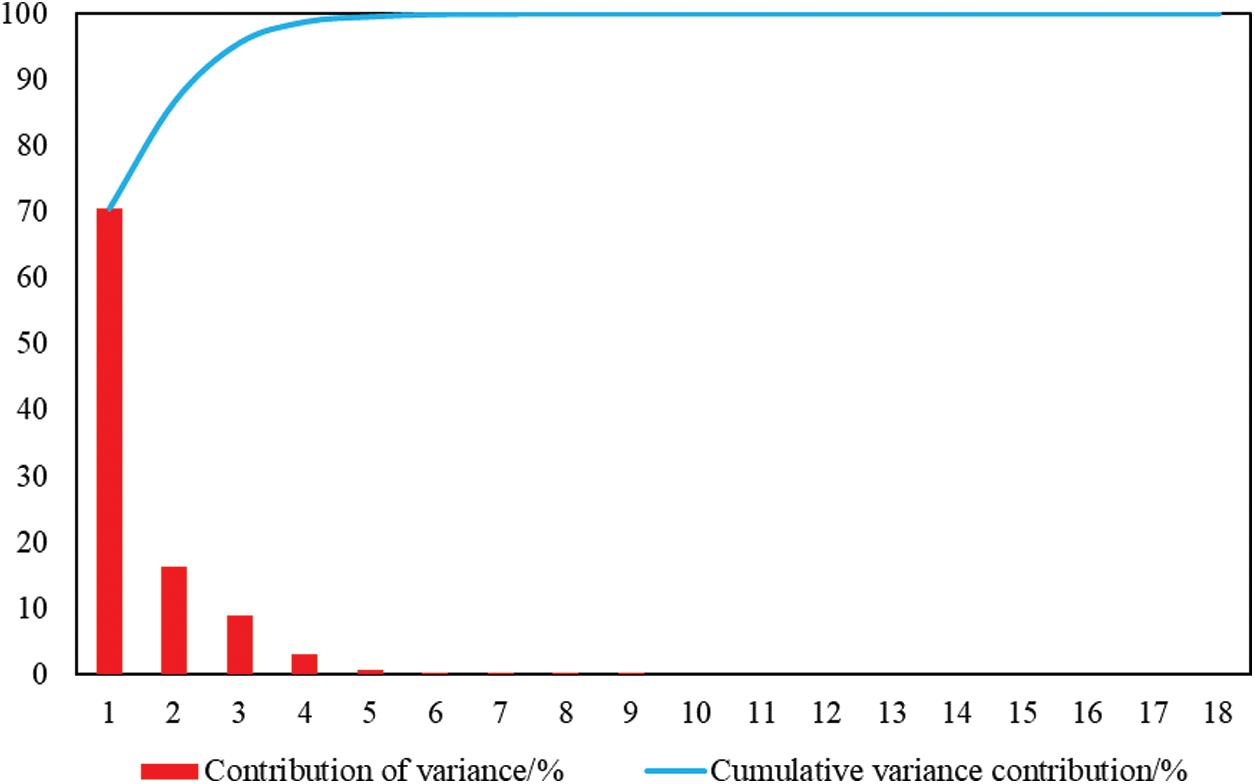
Figure 4: Total variance of KPCA

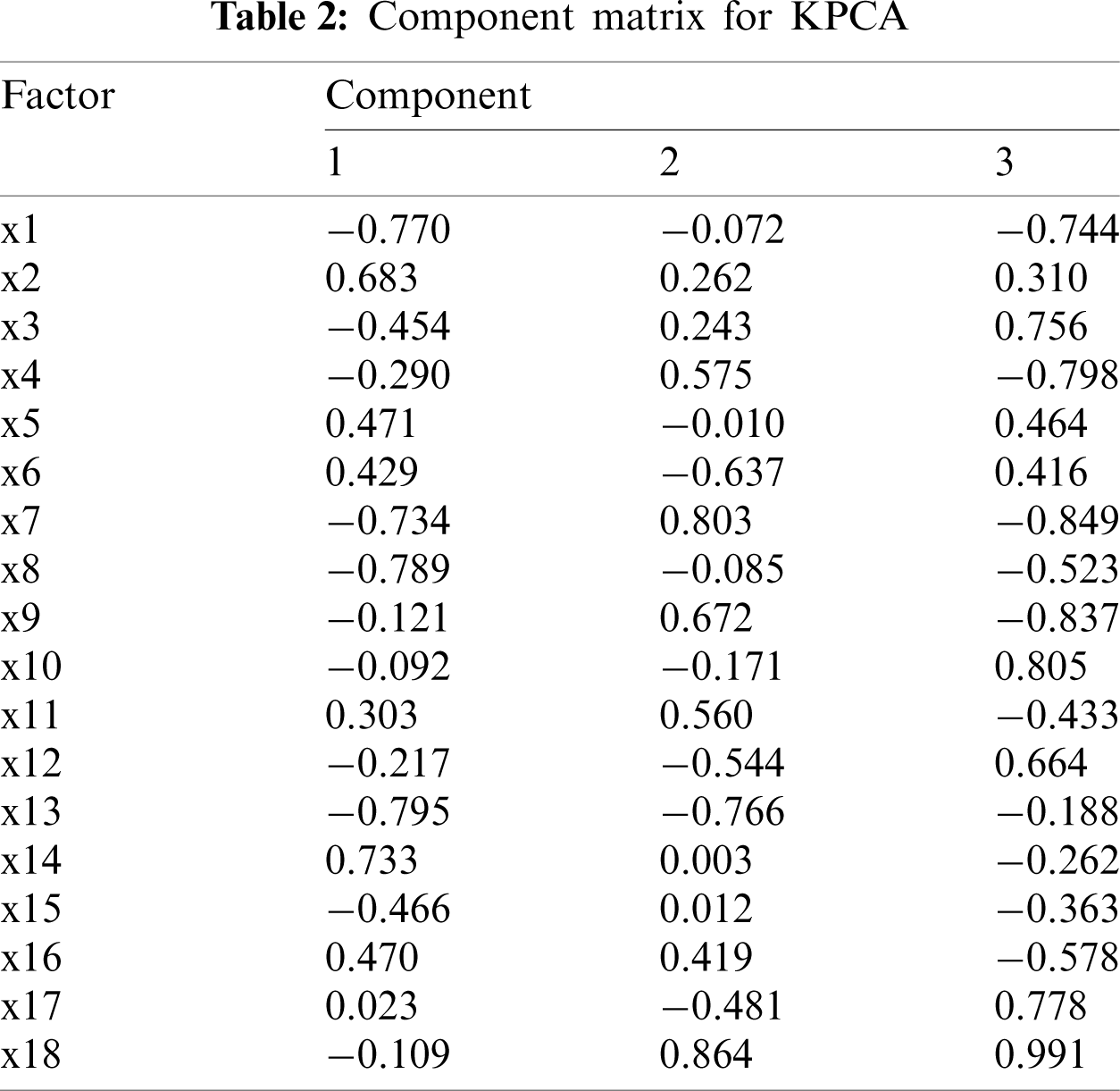
The coefficients of the selected principal components are found by dividing each autonomous component loading vector by the arithmetic square root of the eigenvalues of each autonomous component, and the output component matrix is calculated as displayed in Tab. 2. The components in Tab. 2 form the final input indicators for the prediction model.

4.2 Prediction Results Based on the Proposed Model

This section compares the different forecast effects for the spring, summer, autumn and winter. April 2019, July 2019, October 2019 and January 2020 are taken as representatives of the spring, summer, autumn and winter respectively for forecasting. Eight days are selected as the test sample, and the remaining data are employed as the training sample. Fig. 5 displays the comparison between the actual and predicted PV power values in the test sample set.

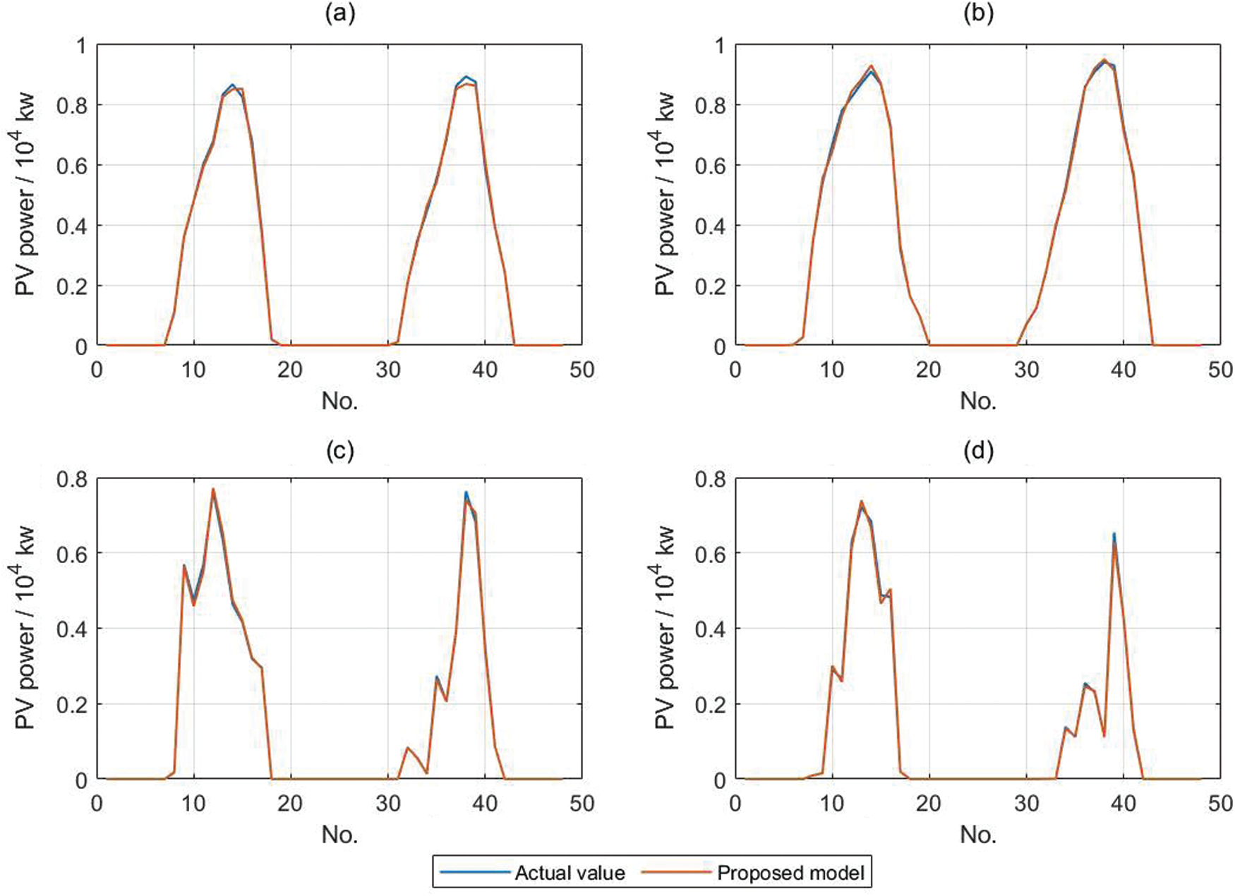
Figure 5: Comparison of PV power prediction results for four seasons: (a) Spring; (b) Summer; (c) Autumn; (d) Winter

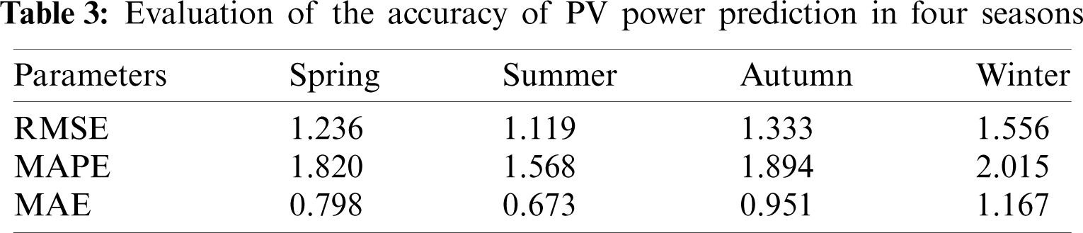
As can be seen in Fig. 5, the PV curve is fuller and smoother in spring and summer. The summer curve is particularly pronounced, mostly on sunny days when the PV output is stable and the power values are high. In autumn, there are spikes and jitters in the PV output due to variable weather, and power values are also generally lower. In winter, the PV curve is narrower, which can be interpreted as shorter sunrise times and shorter maintenance of maximum daily light hours. The RMSE, MAPE and MAE of the test set are shown in Tab. 3, demonstrating the overall prediction effectiveness of the model proposed in this paper. In general, the spring and summer seasons give better predictions, while winter has the worst prediction accuracy, which is in line with our general perception.

4.3 Comparative Analysis

To demonstrate the prediction performance of KPCA-MCS-DCNN, four models, namely MCS-DCNN, CS-DCNN, DCNN and BPNN, are selected for comparison in this paper. The spring test sample is discussed below as an example.

Fig. 6 shows the prediction results of MCS-DCNN, CS-DCNN, DCNN, BPNN and the model proposed in this paper for the PV power test set.

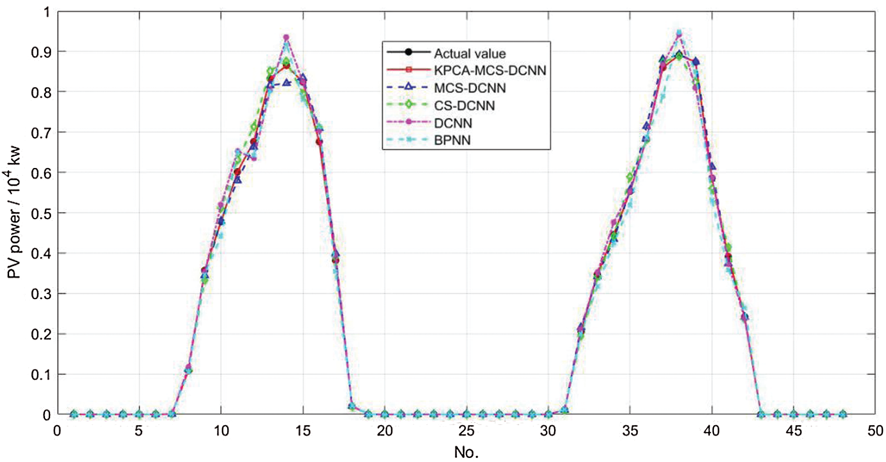
Figure 6: Comparison of predicted results

First, the maximum and minimum relative distances between the actual power values and the predicted values can be seen in Fig. 6. In the BPNN model, the maximum relative distance is 0.071134 and the minimum relative distance is 0.000064; in the DCNN model, the maximum and minimum relative distances are 0.069996 and 0.000059, respectively. Both values of DCNN are smaller than those of BPNN, indicating that the prediction accuracy of DCNN is relatively higher than that of DCNN. In the CS-DCNN model, the maximum and minimum relative distances are 0.049436 and 0.000036, respectively. The difference between the maximum and minimum relative distances is 0.049401, which is smaller than that of the BPNN and DCNN models, indicating that the stability of the CS-DCNN power prediction model is higher than that of the BPNN and DCNN. In the KPCA-MCS-DCNN power prediction model proposed in this paper, the maximum relative distance is only 0.026776, the minimum relative distance is 0.000007, and the deviation between these two distances is only 0.026769. These three values are smaller for the KPCA-MCS-DCNN model compared to the other four prediction models, suggesting that the proposed power prediction model has higher prediction accuracy and superior prediction stability.

Tab. 4 and Fig. 7 demonstrate the RMSE, MAPE and MAE of the individual models for the overall prediction results.

As can be seen from Tab. 4 and Fig. 7, the RMSE of the model proposed in this paper is calculated to be 1.236, while the RMSE of the MCS-DCNN, CS-DCNN, DCNN and BPNN models are calculated to be 1.738, 2.059, 2.825 and 3.354, respectively. This implies that the prediction results of the model proposed in this paper have small errors and the highest overall accuracy of prediction. Similarly, the calculated results of MAPE (1.820) and MAE (0.798) of the KPCA-MCS-DCNN model are both optimal. In short, RMSE, MAPE and MAE of KPCA-MCS-DCNN are all minimum values. It is worth noting that the smaller the values of these three indicators are, the stronger the robustness of the model is. Therefore, it can be concluded that the robustness of KPCA-MCS-DCNN is better. Compared with the MCS-DCNN model, KPCA overcomes the adverse effects of unconventional data on model training caused by sudden changes in the influencing factors. The prediction performance of the MCS-DCNN model is better than that of the CS-DCNN model, indicating that the modified CS algorithm plays a more satisfactory optimization role. The overall prediction performance of the DCNN model is better than that of the BPNN model, indicating that the overall prediction performance of the DCNN model, a type of deep learning algorithm, is significantly superior. Overall, the {KPCA-MCS-DCNN} model has the best prediction performance, followed by the MCS-DCNN model, CS-DCNN model and DCNN model, and the BPNN model has the worst prediction performance.

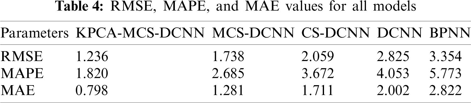
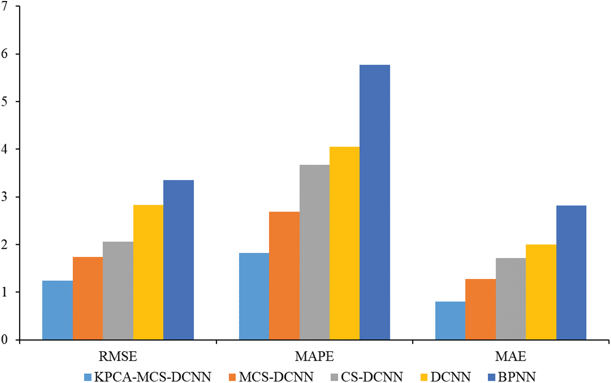
Figure 7: RMSE, MAPE and MAE of the predicted results

In conclusion, the proposed model can effectively reduce the PV power prediction error by optimizing the DCNN model with the MCS algorithm. KPCA model can not only reduce the noise data of the input variables and improve the validity of the input information, but also ensure the integrity of the input information, thus improving the accuracy and robustness of PV power prediction. The effectiveness of the proposed PV power prediction model is demonstrated by the data calculation results.

5  Conclusions and Discussion

Solar energy, as a low operating cost, wide range of applications, inexhaustible, environmentally friendly and harmless renewable energy, has a broad development prospect in the field of electricity. However, the power output of photovoltaic power generation utilizing solar energy as the energy source is greatly influenced by the weather and fluctuates significantly. The instability of PV power has a large impact on the power grid, making it very difficult to plan and control the power system. Consequently, achieving more accurate PV power prediction can effectively help the power sector to make reasonable energy planning and dispatching decisions and promote PV consumption. In this paper, a novel approach for PV power prediction based on KPCA-MCS-DCNN is proposed, in which the key factors are extracted employing KPCA. These key factors are brought into DCNN for learning and training, and MCS is applied to optimize the parameters in DCNN, thereby enhancing its prediction accuracy. An empirical analysis is carried out on a PV plant in China as an example, and MCS-DCNN, CS-DCNN, DCNN and BPNN are selected for comparison with the proposed model. The experimental results verify that the proposed model has better prediction accuracy than the comparison model and can achieve good prediction results, thus providing a new idea and reference for PV power prediction. The main conclusions are summarized as follows:

(1)   The input indexes of the PV power prediction model are downscaled and analyzed by KPCA, while PCA is selected for comparison. It can be concluded that the dimensionality reduction of KPCA is significantly stronger than that of PCA, and KPCA ensures sufficient information of the original data even with fewer principal components.

(2)   The innovative KPCA-MCS-DCNN model is proposed and applied to PV power prediction with RMSE of 1.236, MAPE of 1.820, and MAE of 0.798 in the spring test dataset. On the basis of KPCA to extract principal components, this hybrid model optimizes the DCNN model employing the MCS algorithm. Hence, a complex relationship between input data and PV power is constructed to predict short-term PV power.

(3)   MCS-DCNN, CS-DCNN, DCNN and BPNN are selected for comparison and it is concluded that the proposed power prediction model has higher prediction accuracy and more satisfactory robustness. The different prediction results of spring, summer, autumn and winter seasons are obtained utilizing KPCA-MCS-DCNN and excellent prediction results are all achieved. All of these indicate that the robustness of the proposed model in this paper is better.

In brief, this paper starts from dimensionality reduction of PV power prediction impact factors, and then proposes a hybrid deep learning model based on MCS-DCNN to predict short-term PV power and compares it with other four intelligent prediction models. In future research, more advanced deep learning models can be employed for PV power prediction to obtain more accurate PV power prediction results. In addition, there is room to improve the prediction speed of deep learning models.

Funding Statement: The authors received no specific funding for this study.

Conflicts of Interest: The authors declare that they have no conflicts of interest to report regarding the present study.

This work is licensed under a Creative Commons Attribution 4.0 International License, which permits unrestricted use, distribution, and reproduction in any medium, provided the original work is properly cited.