| Computer Modeling in Engineering & Sciences |
DOI: 10.32604/cmes.2021.016172
ARTICLE
Deep Learning Predicts Stress–Strain Relations of Granular Materials Based on Triaxial Testing Data
1Zienkiewicz Centre for Computational Engineering, College of Engineering, Swansea University, Swansea, Wales, SA1 8EP, UK
2College of Shipbuilding Engineering, Harbin Engineering University, Harbin, 150001, China
3Institute of Applied Mechanics and Biomedical Engineering, Taiyuan University of Technology, Taiyuan, 030024, China
4Fluid Dynamics and Solid Mechanics Group, Theoretical Division, Los Alamos National Laboratory, Los Alamos, NM 87545, USA
*Corresponding Author: Y. T. Feng. Email: y.feng@swansea.ac.uk
Received: 13 February 2021; Accepted: 08 April 2021
Abstract: This study presents an AI-based constitutive modelling framework wherein the prediction model directly learns from triaxial testing data by combining discrete element modelling (DEM) and deep learning. A constitutive learning strategy is proposed based on the generally accepted frame-indifference assumption in constructing material constitutive models. The low-dimensional principal stress-strain sequence pairs, measured from discrete element modelling of triaxial testing, are used to train recurrent neural networks, and then the predicted principal stress sequence is augmented to other high-dimensional or general stress tensor via coordinate transformation. Through detailed hyperparameter investigations, it is found that long short-term memory (LSTM) and gated recurrent unit (GRU) networks have similar prediction performance in constitutive modelling problems, and both satisfactorily predict the stress responses of granular materials subjected to a given unseen strain path. Furthermore, the unique merits and ongoing challenges of data-driven constitutive models for granular materials are discussed.
Keywords: Deep learning; granular materials; constitutive modelling; discrete element modelling; coordinate transformation; LSTM; GRU
Granular materials are ubiquitous in nature, industrial and engineering activities. Predicting how granular materials respond to various external loads is not just intricate but important for many engineering problems. The complexity of granular media can be partially attributed to its unique features, such as inherent anisotropy and heterogeneity [1,2], pressure and rate-dependence [3–5], continuous evolving microstructure and complicated strain-localisation phenomenon within unstable granular materials [6–9].
Over the past decades, analytical or phenomenological characterisation of elastic-plastic behaviour of granular materials is undoubtedly the most common scheme. However, although numerous attempts have been made to capture the constitutive behaviour of granular materials, developing a unified theoretical model remains an ongoing challenge [10]. A pessimistic fact is that phenomenological constitutive models not only are increasingly complex in mathematical forms, but also normally require dozens of parameters to be calibrated. This trend further reduces the possibility of taking these advanced constitutive models into practical engineering applications.
Instead of phenomenological constitutive models, some scholars are seeking a shift of methodology in predicting the constitutive behaviour of granular materials. An attractive alternative is the data-driven paradigm, wherein artificial neural networks (ANNs) are used to train a prediction model directly from observed experimental data, by leveraging the universal approximating capability of deep neural networks for complex mapping relations [11]. Early attempts at using ANNs to predict the stress-strain behaviour of granular materials can be traced back to the literature [12–18]. Owing to the revolutionary development of deep learning in recent years, AI-based constitutive models have again received increasing attention. Wang et al. [19–21] combined deep reinforcement learning and game theory to predict the traction-separation law of interfaces and constitutive behaviour of granular materials. Zhang et al. [22] utilised LSTM to predict the cyclic behaviour of granular materials. Zhang et al. [10] also summarised the applications of machine learning in constitutive modelling of soils. Qu et al. [23] explored several constitutive training strategies by integrating a priori micromechanical knowledge and physics-invariant GRU model.
Overall, the past work mainly focuses on developing advanced learning models or algorithms to learn an accurate prediction model with as few as possible specimens. However, when training a neural network with triaxial testing data and taking these models into practical applications where complex stress-strain states are usually encountered, a direct challenge is how to enable the deep neural networks (DNNs) trained with principal stress-strain data from triaxial testing to predict general stress response in practice.
This work aims to address the above-mentioned challenge by presenting an AI-based constitutive modelling strategy which leverages coordinate transformation to expand the principal strain or stress tensor to a 3D general tensor incorporating shear components. DEM simulations of drained triaxial tests with complex unloading-reloading cycles are used to generate high-fidelity training data. Both LSTM and GRU neural networks are adopted to train the stress-strain prediction models and a detailed hyperparameter investigation process is also presented.
2 Representing Constitutive Relations via Deep Neural Networks
Constitutive models refer to the mathematical formulations which relate the stress responses to strain states of materials at an element level. A state of stress or strain of a point under a general loading condition can be defined by a second-order tensor with 9 components (reduce to 6 components under a symmetry condition). Instead of using any mechanical assumption, DNNs connect these stress components to strain components directly with a series of linear and nonlinear mathematical operations. Since the application of deep learning in predicting the elastic-plastic behaviour of granular materials is still at an early stage of development, an introduction about the fundamentals of a conventional neural network is given in Appendix A.
The constitutive behaviour of materials is essentially a sequence problem. In the family of deep learning, recurrent neural networks (RNNs) are extensions of conventional fully connected neural networks and mainly suitable for sequence data predictions. LSTM and GRU networks are two popular RNNs in dealing with long sequence learning problems. In this study, both networks will be used to train the constitutive models. The detailed internal structures of GRU and LSTM cells and their mathematical operations can be found in [24–26].
2.1 Developing Data-Driven Constitutive Models Based on Triaxial Testing Data
Triaxial tests are commonly used to measure the stress-strain responses of granular materials with the assumption that the triaxial specimen is a representative volume element of the measured materials. Such a loading condition makes the three loading directions happen to be the principal stress/strain directions and the increments of principal stress and strain can be experimentally measured during true triaxial testing. In the process of developing conventional constitutive models, the role of these triaxial tests is to calibrate free parameters and validate the applicability of a new analytical model.
However, when utilising the triaxial testing measurements to train a deep neural network and develop a data-driven constitutive model, some extra work is necessary. The reason is that deep learning can only approximate the mapping between direct inputs (principal strain) and outputs (principal stress), while a constitutive model that can be used to analyse boundary value problems (BVPs) is usually required to incorporate shear stress/strain components. To resolve this issue, a priori knowledge of the frame-indifference (also called the objectivity) will come into play.
Frame-indifference is a generally accepted assumption in the study of constitutive models [27]. It indicates that stress or strain is a physical quantity that is independent of the coordinate frame, although its scalar components depend on the choice of a coordinate reference [28–31]. Therefore the coordinate transformation is a practical strategy to transform the principal stress-strain tensor from triaxial testing to a 3D tensor with full non-zero components. Provided that the whole process of triaxial loading is quasi-static, the coordinate transformation strategy can be applied to the entire stress-strain sequences during testing.
Fig. 1 illustrates the stress transformation between the principal tensor and a 3D tensor incorporating both shear and normal components. Supposing that
where lim and lnj are the cosine angles between two coordinate axes with:
in which em and en are the basis vectors along the xm and xn directions in the first coordinate system;
and its inverse transformation is:
The above formulations can achieve the interchangeable transformation between the principal stress tensor in triaxial testing conditions and a 3D tensor incorporating shear components. The transformation of a strain tensor follows the same rule.
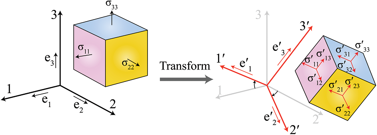
Figure 1: An illustration of stress transformation from principal stress tensor to a 3D tensor incorporating shear components
2.2 Constitutive Learning Strategies Based on Triaxial Testing Data
On the basis of frame indifference, two strategies are available to develop a data-driven constitutive model: one strategy is to perform data augmentation based on the principal stress-strain pairs by rotating the original coordinate frame. Depending on the selected interval of the rotation angle, thousands of data specimens incorporating normal and shear components can be artificially generated based on simply one principal stress-strain sequence pair. Then all the augmented data specimens are used to train the deep neural networks. In this case, the AI model will naturally achieve the aim of predicting stress responses with a 3D strain tensor incorporating both shear and normal components. As the strategy augments data first and then training models later, we would name it as “Augmentation First and Training Later,” short for “AFTL.” The basic workflow of the AFTL strategy can be found in Fig. 2.
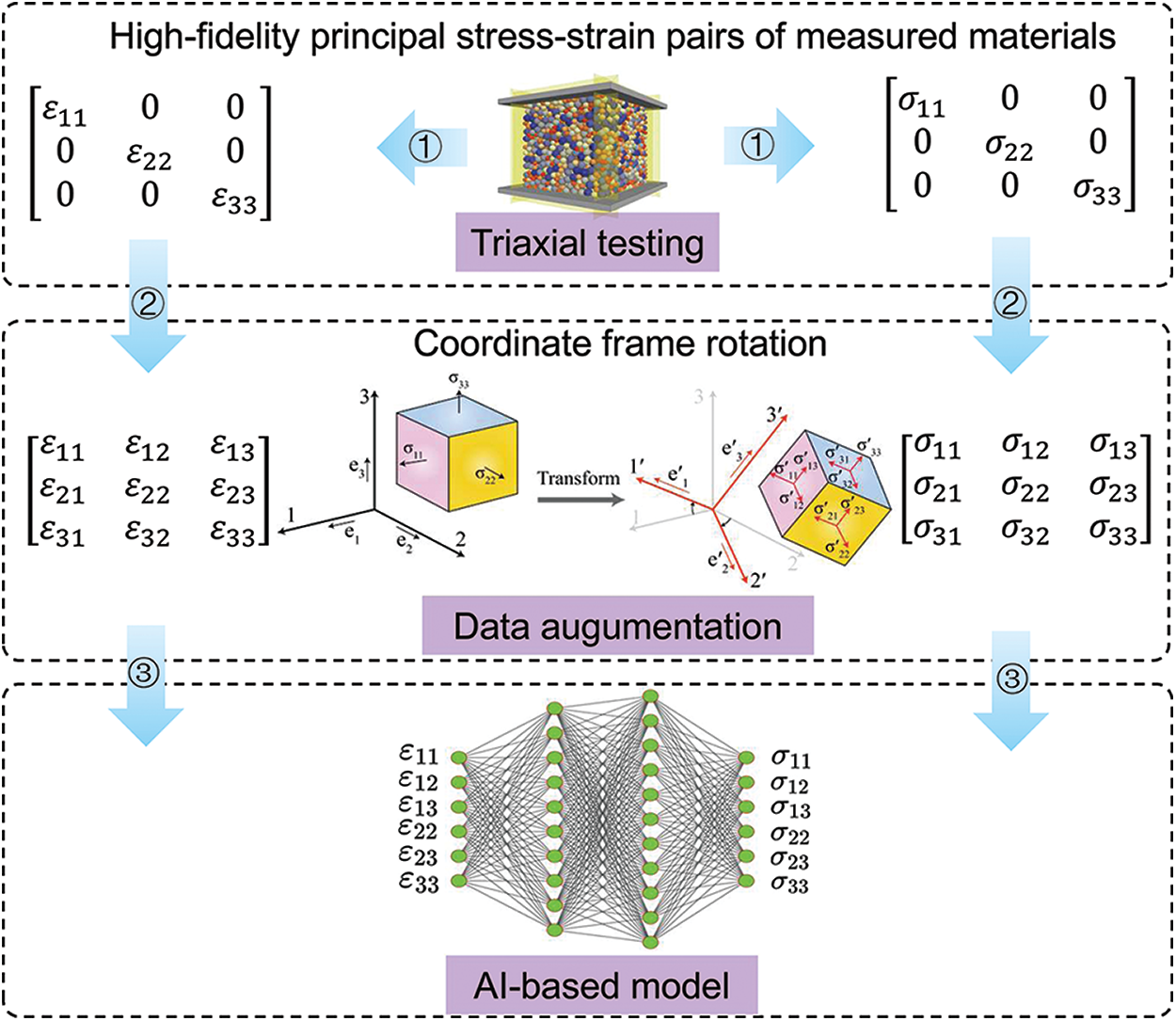
Figure 2: The basic workflow of AFTL strategy
The other strategy is to train the neural networks only with the principal stress and strain data. Fig. 3 illustrates the basic procedure of this strategy for developing a data-driven model. During the training phase, the first step is to obtain principal stress and strain pairs via experimental or numerical triaxial testing. The second step is to train the deep neural network based on the triaxial data. In the usage phase, before putting the data-driven model into macroscopic modelling for a BVP problem, the strain state experienced by each computational element is required to transform to the corresponding principal strain form, using a similar formula to Eq. (4) (replacing the stress quantity with a strain quantity). The trained DNN receives the transformed principal strain tensor as inputs and produces the corresponding principal stress components as outputs. By leveraging the derived transformation matrix obtained in transforming a general strain tensor to the principal strain tensor, the predicted principal stress tensor can be converted back to a general stress tensor
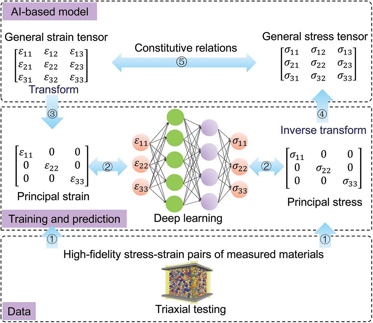
Figure 3: The basic workflow of TFAL strategy
Recalling the fact that the coordinate transformation does not change the stress or strain state experienced by a point, all these artificially generated specimens essentially represent the identical state as the original one. Therefore the AFTL strategy may include information redundancy. Inevitably a marked increase in the number of training specimens will give rise to a far greater DNN scale and a larger training cost. Besides, the choice of the interval of rotation angle becomes a new hyperparameter that has to be artificially tuned. By contrast, the TFAL strategy avoids these downsides and is thus recommended as a preferred scheme in this study.
3 Implementing Data-Driven Constitutive Models Based on Triaxial Testing Data
3.1 Data Preparation via Discrete Element Modelling of Triaxial Testing
As a high-dimensional surrogate model, deep learning normally requires a large amount of data to train the model. Laboratory experiments are not only expensive but time-consuming. In contrast, DEM has proven to be capable of capturing the salient behaviour of real granular materials [32–37]. It is thus feasible to use DEM to develop a data-driven constitutive model. Because a general loading condition may require thousands of test specimens, here we focus on the ability of the data-driven model in predicting multiple unloading-reloading cycles and restrict the simulation to a conventional triaxial testing environment with a state of constant confining stress.
In this study, a total of 220 numerical triaxial specimens with 4037 spherical particles for each model are generated via DEM. The particle radii are uniformly distributed between 2 and 4 mm. The normal and tangential contact stiffnesses, interparticle frictional coefficient, particle density, viscous damping ratio are 105 N/m,
3.2 Constructing Deep Learning Models for Constitutive Modelling
Before training, all the data specimens from DEM are transformed with the MinMaxScaler in the scikit-learn package to scale each feature to a range of (0,1). This transformation of data benefits reducing the risk of getting stuck in local optima and makes the training process faster. Then the scaled data specimens are shuffled with a certain random seed. The whole specimens are partitioned into training, validation, and test datasets with 96, 24, and 100 groups of datasets, respectively. These specimens are mutually different and never seen for each other.
The LSTM and GRU neural networks are built on Tensorflow platform with Nvidia GPU accelerated computation framework for all the training process. The prediction accuracy of the deep learning models is evaluated by the scaled mean absolute error (SMAE), which is used as the cost function when training a DNN model and also the metric to evaluate the final trained model. The formula of an average SMAE can be calculated by:
where SMAE represents the average value of SMAE for all the stress-strain curves; Nj and N are the number of data points on the jth stress-strain curve and the number of stress-strain curves, respectively;
3.3 Hyperparameter Investigation
The approximation capability of a deep learning model is related to its used architecture and network configuration. To explore a suitable network configuration for the current constitutive modelling problem in this work, a detailed parametric study is conducted. The preliminary network configuration starts from one or two RNN layers, followed by one or zero dense layer, before connecting the output layer. The neuron number in each hidden layer varies from 0 to 120 with a gap of 20. The final network architecture will be determined by comprehensively considering (1) the amount of SMAE, and (2) the complexity of architectures. Specifically, if the difference of two SMAEs is within 10−5, the simplest architecture with the least parameters to be trained will be selected because a simpler model has less risk of overfitting. The SMAEs of different network architectures can be found in Fig. 4 and the architectures [LSTM:100-LSTM:100-dense:0] and [GRU:100-dense:0] are finally selected for LSTM and GRU neural networks, respectively. The LSTM model trains 122,101 weights and biases (41,600 parameters for the first LSTM layer; 80,400 parameters for the second LSTM layer, and the output layer includes 121 parameters). The GRU model requires a total of 31,301 weights and biases to be learned with 31,200 parameters for the GRU layer and 101 parameters for the output layer.
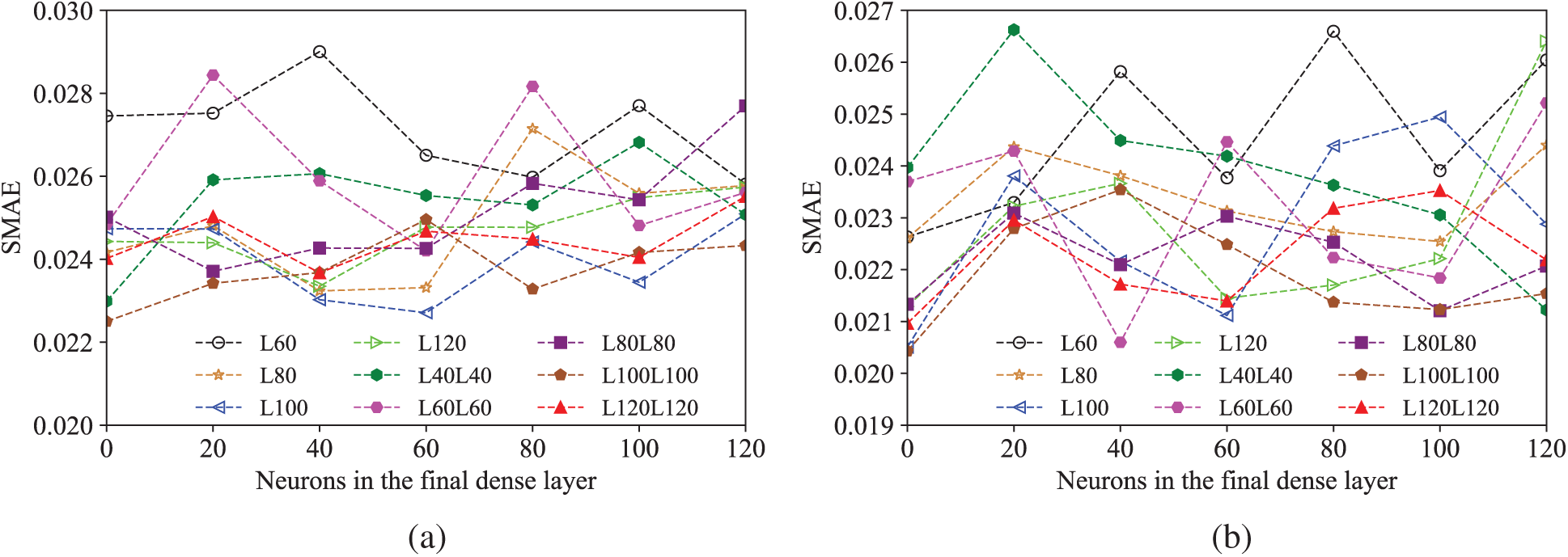
Figure 4: Parametric investigation of the RNN neural network configurations (a) LSTM (b) GRU
After a suitable network configuration has been selected, the next step is to train the network to fully exploit the prediction ability of this surrogate model. Therefore, the influences of some other important hyperparameters (e.g., timesteps, batch size and learning rate) should be considered. Empirically, the batch size is usually selected from a power of 2 (e.g., 2n); the learning rate normally starts from 0.001 and increases to 0.01 and 0.1.
With all these considerations, an investigation of SMAE against different timesteps and batch sizes is shown in Fig. 5. It is found that the SMAE value of a trained model decreases with an increase in the timesteps but this tendency slows down for the timesteps over a certain value. Considering that a larger timestep gives rise to a larger computational cost, the optimal time step for both LSTM and GRU is selected as 40. On the other hand, the influences of the learning rate and the batch size on the prediction results seem limited for both GRU and LSTM models. Based on the parametric investigation, the final hyperparameter combinations of the LSTM model and the GRU model are: [timesteps: 40, batch size: 32, learning rate: 0.001] and [timesteps: 40, batch size: 64, learning rate: 0.001], respectively.
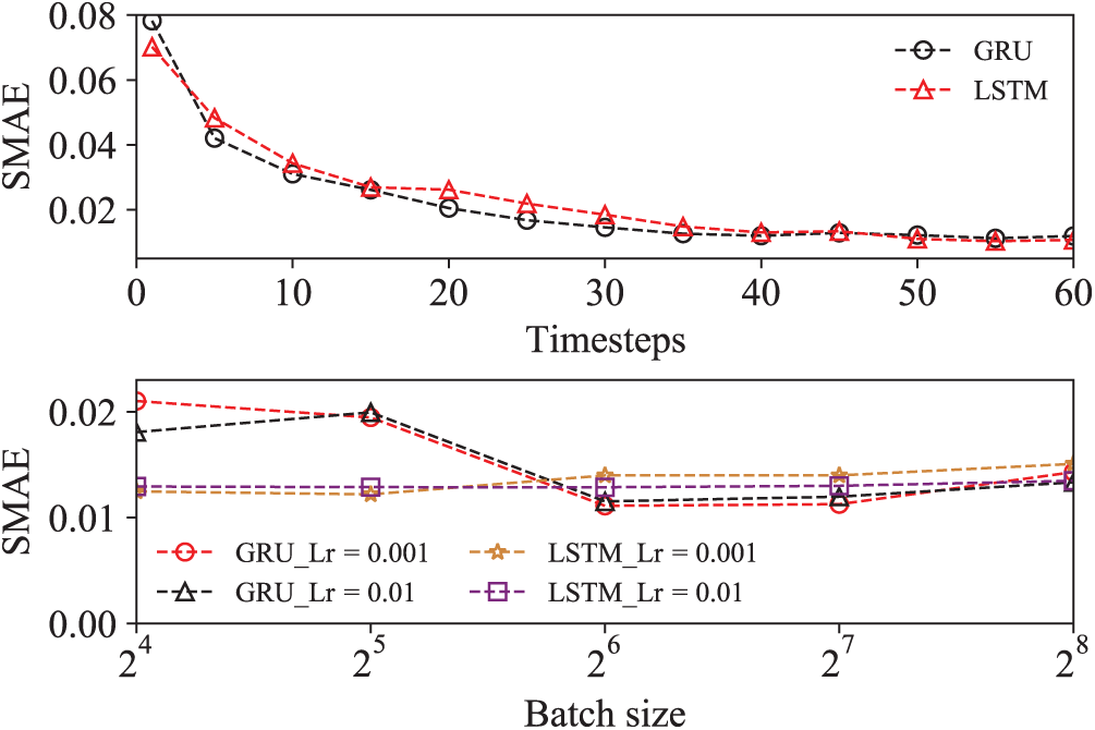
Figure 5: SMAEs of the selected LSTM and GRU models against various timesteps and batch size
The learning curves of both LSTM and GRU models with the selected hyperparameters are shown in Fig. 6, which demonstrates that LSTM and GRU have a similar prediction accuracy in the current constitutive modelling problem. Specifically, LSTM seems to converge quicker at the early training epochs but the prediction difference shrinks later on. To determine the architecture and hyperparameters of the final training models, a total of 87 groups of distinct training configurations for each RNN model are considered.
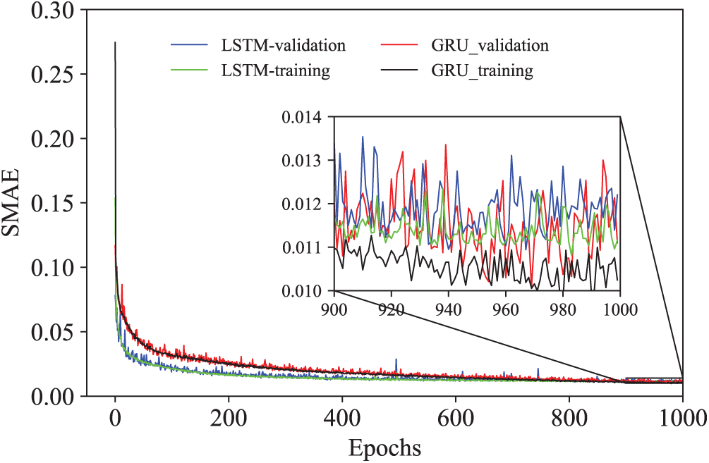
Figure 6: The learning curves of the selected LSTM and GRU models
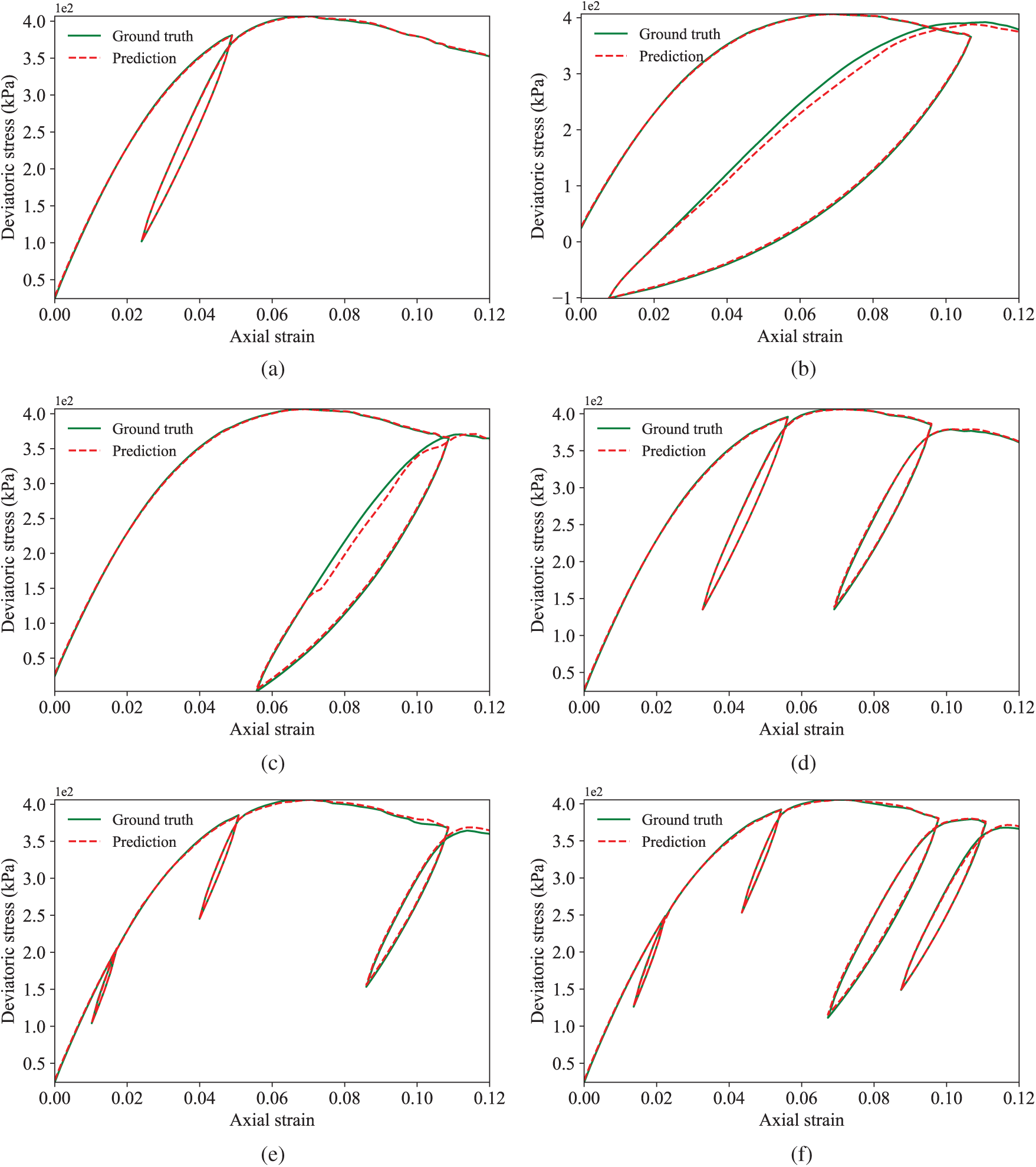
Figure 7: Representative prediction results of the trained LSTM model (a) The best prediction, SMAE:0.007 (b) The worst prediction, SMAE:0.051 (c) The second worst prediction, SMAE:0.048 (d) Two unloading-reloading cycles, SMAE:0.018 (e) Three unloading-reloading cycles, SMAE:0.016 (f) Four unloading-reloading cycles, SMAE:0.015
Note that the hyperparameter selection for a deep neural network is essentially a very high dimensional combinatorial optimisation problem, it is thus not easy to search all the possible combinations considering available computational resources. Although the parametric study does not cover many combinations, it provides a relatively reliable network configuration and parameters for the model in the searched parameter space.
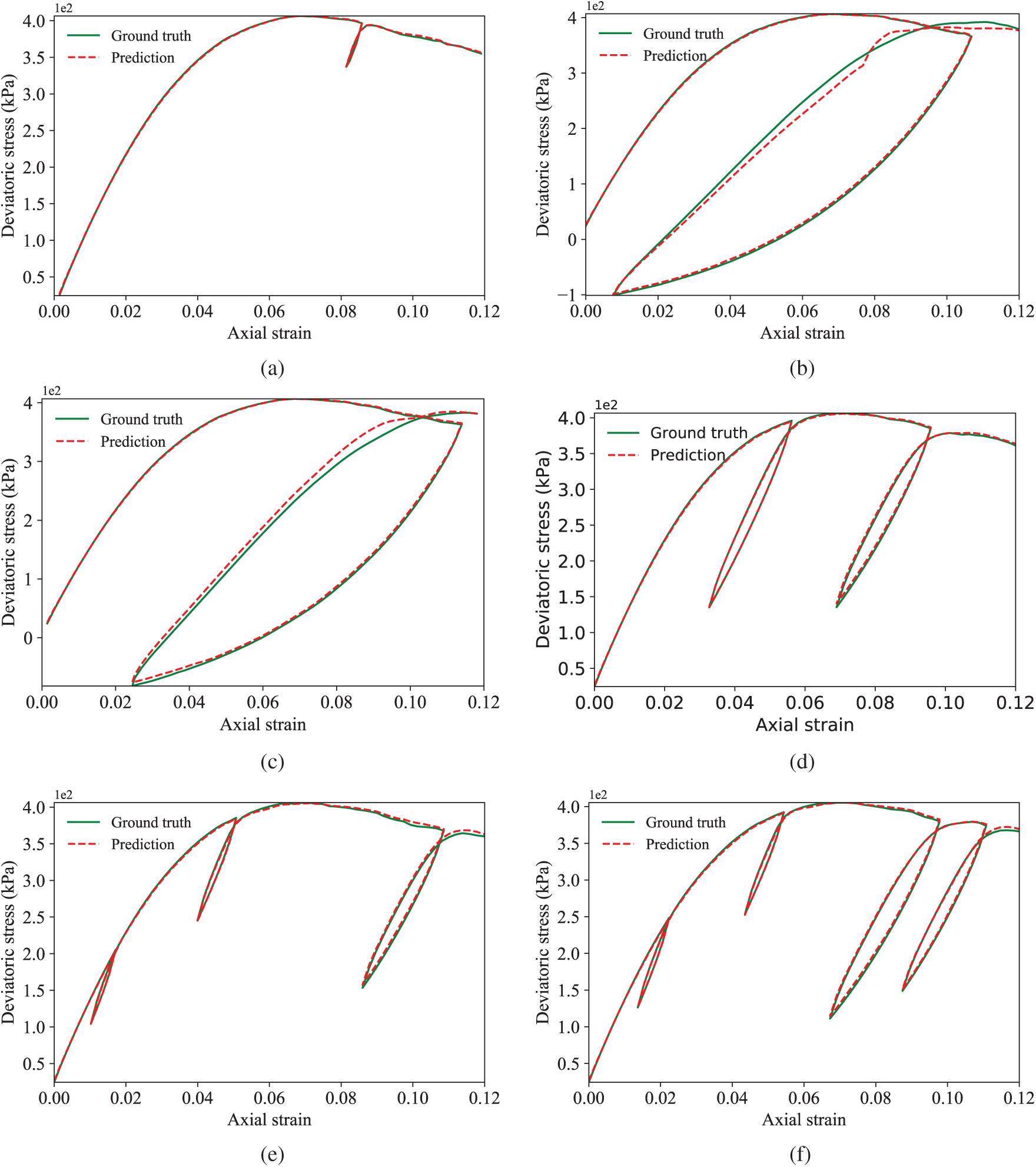
Figure 8: Representative prediction results of the trained GRU model (a) The best prediction, SMAE:0.007 (b) The worst prediction, SMAE:0.054 (c) The second worst prediction, SMAE:0.044 (d) Two unloading-reloading cycles, SMAE:0.017 (e) Three unloading-reloading cycles, SMAE:0.017 (f) Four unloading-reloading cycles, SMAE:0.014
3.4 The Prediction Performance of an AI-Based Constitutive Models
The LSTM model predicts the 100 groups of unseen test specimens with an average SMAE of 0.0193. The smallest SMAE is 0.007 and the largest SMAE is 0.051. For the GRU model, the average SMAE on the test specimens is 0.0189. The best prediction has a SMAE of 0.007, while the worst prediction has a SMAE of 0.054. Some typical predictions given by the trained LSTM and GRU model are shown in Figs. 7 and 8, respectively.
On the one hand, the results confirm that the LSTM and GRU have similar prediction performances on the stress-strain behaviour of granular materials. On the other hand, it is found that even for the worst and the second worst prediction cases, the overall tendency of stress responses has been satisfactorily captured by both LSTM and GRU models. The results demonstrate that the prediction accuracy of the trained model is acceptable and the DNN model is able to predict complex cases with more than two unloading-reloading cycles, which is very challenging to achieve for phenomenological constitutive models.
Conventional continuum-based elastic-plastic constitutive models normally utilise 1) yield surfaces to describe plasticity, and 2) associative or non-associative flow rules to characterise the evolution direction of plastic deformation. This work offers an alternative to currently used phenomenological models for granular materials by training a data-driven constitutive model via RNN neural networks based on triaxial testing data. The work adopts coordinate transformation to transform the principal stress or strain tensor to a general 3D tensor incorporating both normal and shear components, and a constitutive training strategy is summarised. Also, both LSTM and GRU neural networks are used to train the stress-strain prediction model. The results demonstrate that the LSTM and GRU models have a similar prediction accuracy and both of them are powerful in predicting the macroscopic elastic-plastic responses of granular materials.
The data-driven paradigm has unique advantages in the constitutive modelling of materials. First, it can be embedded in macroscopic numerical modelling (such as FEM or MPM) for practical applications without extra simplifications. Second, its prediction ability can be further improved, provided that new data specimens are added. Third, the DNN model is capable of predicting complex stress-strain responses with excellent accuracy and efficiency. It not only inherits the merits of DEM in naturally capturing stress-strain relations of granular materials undergoing large deformation and shear localisation, but overwhelmingly accelerates the stress-strain predictions given by ab initio DEM. Therefore, the data-driven constitutive model may have potentials to address some dilemmas which traditional constitutive models struggle with.
It should be noted that constitutive models for a specific granular material should be associated with its material and state parameters, such as particle size distribution, mineralogical compositions and porosity etc. More advanced deep learning models considering these physics-invariant properties can be found in [23]. The other important issue is that granular materials subjected to complex plastic deformation are of non-coaxial behaviour between the principal stress directions and plastic strain rate directions. A further extension on the current framework by incorporating non-coaxiality will be reported elsewhere.
Funding Statement: This work is partially supported by the National Natural Science Foundation of China (NSFC) (Grant Nos. 41606213, 51639004 and 12072217).
Conflicts of Interest: The authors declare that they have no conflicts of interest to report regarding the present study.
1. Ueda, K., Iai, S. (2019). Constitutive modeling of inherent anisotropy in a strain space multiple mechanism model for granular materials. International Journal for Numerical and Analytical Methods in Geomechanics, 43(3), 708–737. DOI 10.1002/nag.2883. [Google Scholar] [CrossRef]
2. Petalas, A. L., Dafalias, Y. F., Papadimitriou, A. G. (2020). Sanisand-f: Sand constitutive model with evolving fabric anisotropy. International Journal of Solids and Structures, 188(3), 12–31. DOI 10.1016/j.ijsolstr.2019.09.005. [Google Scholar] [CrossRef]
3. Li, X. S., Dafalias, Y. F., Wang, Z. L. (1999). State-dependant dilatancy in critical-state constitutive modelling of sand. Canadian Geotechnical Journal, 36(4), 599–611. DOI 10.1139/t99-029. [Google Scholar] [CrossRef]
4. Gudehus, G. (1996). A comprehensive constitutive equation for granular materials. Soils and Foundations, 36(1), 1–12. DOI 10.3208/sandf.36.1. [Google Scholar] [CrossRef]
5. Das, S. K., Das, A. (2019). Influence of quasi-static loading rates on crushable granular materials: A DEM analysis. Powder Technology, 344, 393–403. DOI 10.1016/j.powtec.2018.12.024. [Google Scholar] [CrossRef]
6. Desrues, J., Andò, E. (2015). Strain localisation in granular media. Comptes Rendus Physique, 16(1), 26–36. DOI 10.1016/j.crhy.2015.01.001. [Google Scholar] [CrossRef]
7. Dafalias, Y. F. (2016). Must critical state theory be revisited to include fabric effects? Acta Geotechnica, 11(3), 479–491. DOI 10.1007/s11440-016-0441-0. [Google Scholar] [CrossRef]
8. Qu, T., Feng, Y., Wang, Y., Wang, M. (2019). Discrete element modelling of flexible membrane boundaries for triaxial tests. Computers and Geotechnics, 115(7), 103154. DOI 10.1016/j.compgeo.2019.103154. [Google Scholar] [CrossRef]
9. Qu, T., Feng, Y., Wang, M. (2021). An adaptive granular rve model with an evolutionary periodic boundary for hierarchical multiscale analysis. International Journal for Numerical Methods in Engineering, 122(9), 2239–2253. DOI 10.1002/nme.6620. [Google Scholar] [CrossRef]
10. Zhang, P., Yin, Z. Y., Jin, Y. F. (2021). State-of-the-art review of machine learning applications in constitutive modeling of soils. Archives of Computational Methods in Engineering, 1–26. DOI 10.1007/s11831-020-09524-z. [Google Scholar] [CrossRef]
11. Hornik, K., Stinchcombe, M., White, H. (1989). Multilayer feedforward networks are universal approximators. Neural Networks, 2(5), 359–366. DOI 10.1016/0893-6080(89)90020-8. [Google Scholar] [CrossRef]
12. Ellis, G., Yao, C., Zhao, R., Penumadu, D. (1995). Stress-strain modeling of sands using artificial neural networks. Journal of Geotechnical Engineering, 121(5), 429–435. DOI 10.1061/(ASCE)0733-9410(1995)121:5(429). [Google Scholar] [CrossRef]
13. Ghaboussi, J., Sidarta, D. (1998). New nested adaptive neural networks (NANN) for constitutive modeling. Computers and Geotechnics, 22(1), 29–52. DOI 10.1016/S0266-352X(97)00034-7. [Google Scholar] [CrossRef]
14. Shin, H., Pande, G. (2000). On self-learning finite element codes based on monitored response of structures. Computers and Geotechnics, 27(3), 161–178. DOI 10.1016/S0266-352X(00)00016-1. [Google Scholar] [CrossRef]
15. Javadi, A., Tan, T., Zhang, M. (2003). Neural network for constitutive modelling in finite element analysis. Computer Assisted Mechanics and Engineering Sciences, 10(4), 523–530. DOI 10.1.1.519.6806. [Google Scholar]
16. Hashash, Y., Jung, S., Ghaboussi, J. (2004). Numerical implementation of a neural network based material model in finite element analysis. International Journal for Numerical Methods in Engineering, 59(7), 989–1005. DOI 10.1002/nme.905. [Google Scholar] [CrossRef]
17. Banimahd, M., Yasrobi, S., Woodward, P. K. (2005). Artificial neural network for stress-strain behavior of sandy soils: Knowledge based verification. Computers and Geotechnics, 32(5), 377–386. DOI 10.1016/j.compgeo.2005.06.002. [Google Scholar] [CrossRef]
18. Jung, S., Ghaboussi, J. (2006). Neural network constitutive model for rate-dependent materials. Computers & Structures, 84(15–16), 955–963. DOI 10.1016/j.compstruc.2006.02.015. [Google Scholar] [CrossRef]
19. Wang, K., Sun, W. (2019). Meta-modeling game for deriving theory-consistent, microstructure-based traction-separation laws via deep reinforcement learning. Computer Methods in Applied Mechanics and Engineering, 346(2), 216–241. DOI 10.1016/j.cma.2018.11.026. [Google Scholar] [CrossRef]
20. Wang, K., Sun, W., Du, Q. (2019). A cooperative game for automated learning of elasto-plasticity knowledge graphs and models with ai-guided experimentation. Computational Mechanics, 64(2), 467–499. DOI 10.1007/s00466-019-01723-1. [Google Scholar] [CrossRef]
21. Wang, K., Sun, W., Du, Q. (2021). A non-cooperative meta-modeling game for automated third-party calibrating, validating and falsifying constitutive laws with parallelized adversarial attacks. Computer Methods in Applied Mechanics and Engineering, 373(1), 113514. DOI 10.1016/j.cma.2020.113514. [Google Scholar] [CrossRef]
22. Zhang, P., Yin, Z. Y., Jin, Y. F., Ye, G. L. (2020). An ai-based model for describing cyclic characteristics of granular materials. International Journal for Numerical and Analytical Methods in Geomechanics, 44(9), 1315–1335. DOI 10.1002/nag.3063. [Google Scholar] [CrossRef]
23. Qu, T., Di, S., Feng, Y., Wang, M., Zhao, T. T. (2021). Towards data-driven constitutive modelling for granular materials via micromechanics-informed deep learning. International Journal of Plasticity. Under Review. [Google Scholar]
24. Hochreiter, S., Schmidhuber, J. (1997). Long short-term memory. Neural Computation, 9(8), 1735–1780. DOI 10.1162/neco.1997.9.8.1735. [Google Scholar] [CrossRef]
25. Cho, K., Van Merriënboer, B., Gulcehre, C., Bahdanau, D., Bougares, F. et al. (2014). Learning phrase representations using RNN encoder-decoder for statistical machine translation. arXiv preprint arXiv: 1406.1078. [Google Scholar]
26. Mozaffar, M., Bostanabad, R., Chen, W., Ehmann, K., Cao, J. et al. (2019). Deep learning predicts path-dependent plasticity. Proceedings of the National Academy of Sciences of the United States of America, 116(52), 26414–26420. DOI 10.1073/pnas.1911815116. [Google Scholar] [CrossRef]
27. Tobita, Y. (1989). Fabric tensors in constitutive equations for granular materials. Soils and Foundations, 29(4), 91–104. DOI 10.3208/sandf1972.29.4_91. [Google Scholar] [CrossRef]
28. Liu, I. S. (2011). Constitutive theories: Basic principles. Continuum Mechanics, Encyclopedia of Life Support Systems, 1, 198. [Google Scholar]
29. Liu, I. S., Sampaio, R. (2014). Remarks on material frame-indifference controversy. Acta Mechanica, 225(2), 331–348. DOI 10.1007/s00707-013-0973-4. [Google Scholar] [CrossRef]
30. Hu, N., Yu, H. S., Yang, D. S., Zhuang, P. Z. (2019). Constitutive modelling of granular materials using a contact normal-based fabric tensor. Acta Geotechnica, 15(5), 1–27. DOI 10.1007/s11440-019-00811-z. [Google Scholar] [CrossRef]
31. Sitharam, T. G., Dinesh, S., Shimizu, N. (2002). Micromechanical modelling of monotonic drained and undrained shear behaviour of granular media using three-dimensional DEM. International Journal for Numerical and Analytical Methods in Geomechanics, 26(12), 1167–1189. DOI 10.1002/nag.240. [Google Scholar] [CrossRef]
32. O’Sullivan, C. (2011). Particulate discrete element modelling: A geomechanics perspective. London: CRC Press. [Google Scholar]
33. Gong, J., Nie, Z., Zhu, Y., Liang, Z., Wang, X. (2019). Exploring the effects of particle shape and content of fines on the shear behavior of sand-fines mixtures via the dem. Computers and Geotechnics, 106(3–4), 161–176. DOI 10.1016/j.compgeo.2018.10.021. [Google Scholar] [CrossRef]
34. Gong, J., Liu, J., Cui, L. (2019). Shear behaviors of granular mixtures of gravel-shaped coarse and spherical fine particles investigated via discrete element method. Powder Technology, 353(5), 178–194. DOI 10.1016/j.powtec.2019.05.016. [Google Scholar] [CrossRef]
35. Qu, T., Feng, Y., Zhao, T., Wang, M. (2019). Calibration of linear contact stiffnesses in discrete element models using a hybrid analytical-computational framework. Powder Technology, 356, 795–807. DOI 10.1016/j.powtec.2019.09.016. [Google Scholar] [CrossRef]
36. Qu, T., Wang, S., Fu, J., Hu, Q., Zhang, X. (2019). Numerical examination of EPB shield tunneling-induced responses at various discharge ratios. Journal of Performance of Constructed Facilities, 33(3), 4019035. DOI 10.1061/(ASCE)CF.1943-5509.0001300. [Google Scholar] [CrossRef]
37. Qu, T., Feng, Y., Wang, M., Jiang, S. (2020). Calibration of parallel bond parameters in bonded particle models via physics-informed adaptive moment optimisation. Powder Technology, 366, 527–536. DOI 10.1016/j.powtec.2020.02.077. [Google Scholar] [CrossRef]
Appendix A. Fundamentals of Deep Learning
Deep learning is a subset of machine learning based on deep (multiple-layer) artificial neural networks (ANNs). As shown in Fig. A.1, a deep neural network (DNN) is generally composed of one input layer, several hidden layers, and one output layer. The input layer receives input values (independent variables) and passes them on to the hidden layers while the output layer produces the prediction results (estimated values of dependent variables).
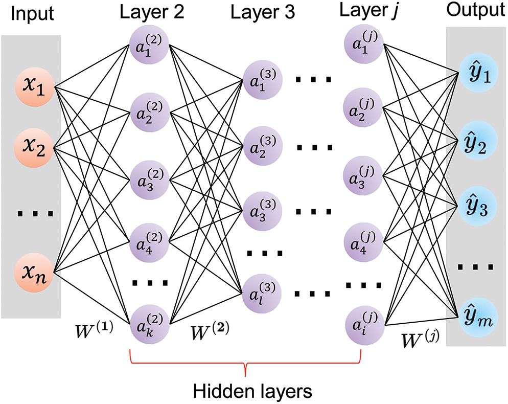
Figure A.1: Diagram of deep neural networks
Fig. A.2 illustrates the basic procedure of deep learning. The process of feeding input data through the network and outputting prediction results is called forward propagation. Mathematically, the forward propagation of a deep neural network is a combination of a series of linear transformations with matrix multiplication and nonlinear transformations with activation functions. In Fig. A.1, the values of the activation functions in each neuron are:
where
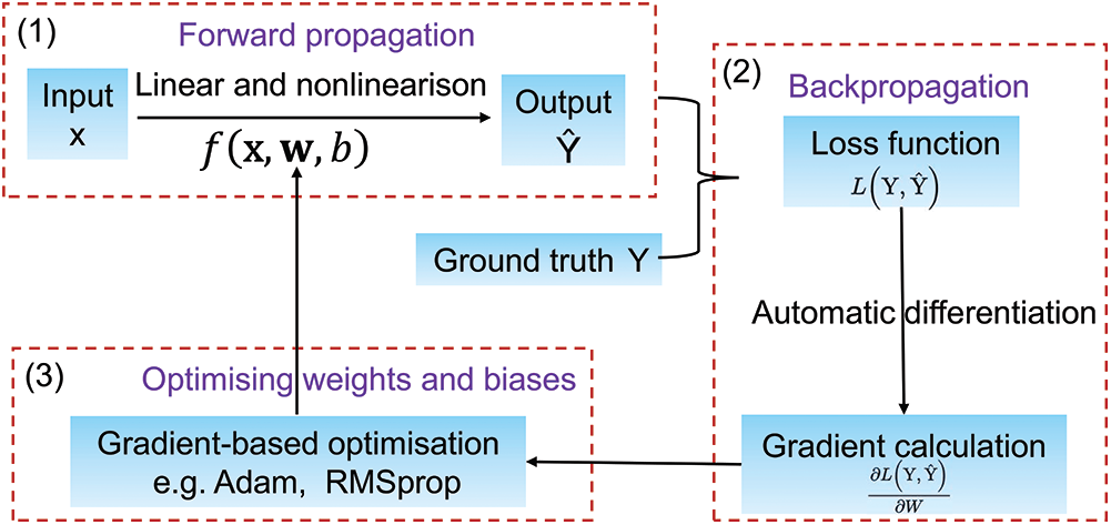
Figure A.2: Diagram of deep learning procedures
Assuming that the jth layer is the last hidden layer, the prediction outputs
where d is the number of neurons in the last hidden layer, and f is the activation function in the output layer. For a trained model, the weights and biases of a network are known. The final prediction results can be explicitly calculated via the forward propagation.
The nature of deep learning is to discover a hypothesis function or “surrogate model” based on DNNs’ architectures to represent a certain mapping or relation. Initially, the weights and biases in DNN are randomly initialised. The resulting prediction by the forward propagation will normally be far away from the ground truth. The difference between the prediction and the ground truth is quantified by a loss function. For a prescribed neural network structure, the loss function is specified as a function of weights and biases.
To train a reliable hypothesis model, the learning problem is converted to an optimisation problem with the target of minimising the loss function. Normally, the network weights and biases are iteratively optimised by a gradient-based optimisation algorithm, e.g., gradient descent. The required gradients are calculated by the backpropagation algorithm, which utilises automatic differentiation (AD) to numerically evaluate the derivative of a function by applying the chain rule repeatedly to the elementary arithmetic operations constituting the loss function.
In the training phase, the optimised weights and biases are used for the next forward propagation to update the loss function. Then the backpropagation and the gradient-based optimisation algorithm further adjust the weights and biases for the next forward propagation. After the process is repeated for a sufficiently large number of training cycles, the neural network will usually be able to predict the results satisfactorily. Then the weights and network architectures can be saved for future use.
 | This work is licensed under a Creative Commons Attribution 4.0 International License, which permits unrestricted use, distribution, and reproduction in any medium, provided the original work is properly cited. |