| Computer Modeling in Engineering & Sciences |
DOI: 10.32604/cmes.2021.015472
ARTICLE
Modeling Dysentery Diarrhea Using Statistical Period Prevalence
Department of Nuclear Engineering, College of Engineering, King Abdulaziz University, Jeddah, 21589, Saudi Arabia
*Corresponding Author: Fouad A. Abolaban. Email: fabolaban@kau.edu.sa
Received: 21 December 2020; Accepted: 07 February 2021
Abstract: Various epidemics have occurred throughout history, which has led to the investigation and understanding of their transmission dynamics. As a result, non-local operators are used for mathematical modeling in this study. Therefore, this research focuses on developing a dysentery diarrhea model with the use of a fractional operator using a one-parameter Mittag–Leffler kernel. The model consists of three classes of the human population, whereas the fourth one belongs to the pathogen population. The model carefully deals with the dimensional homogeneity among the parameters and the fractional operator. In addition, the model was validated by fitting the actual number of dysentery diarrhea infected cases covering 52 weeks in 2017, which occurred in Ethiopia. The biological parameters were fitted, and fractional order
Keywords: Dysentery diarrhea model; Mittag–Leffler kernel; fractional operator
The literature provides mathematical models for the transmission of infectious diseases. These models play a significant role in quantifying and evaluating the effective control and preventive measures of infectious diseases [1–3]. Furthermore, mathematical modeling has been used in several ways as a versatile and effective way of studying the dynamics of infectious disease transmission. This can include the classic susceptible, infected, and recovered (SIR) model or more advanced models [4]. Mathematical analysis and numerical simulations can be collectively used for the development and evaluation of persuasive control measures.
It is popularly known that mathematical models can predict the emergence of infectious diseases and epidemics, which are beneficial for public health planning and initiatives. By using compartmental models as a simple mathematical structure, the complex dynamics of epidemiological processes can be examined [5]. These compartmental models divide the population into two distinct health categories. The first category is depicted by S, and involves those susceptible to pathogen infection, while the second, denoted by I, involves the pathogen-infected humans. The manner in which these two populations interact is based on phenomenological assumptions used to develop the models. Ordinary differential equations (ODEs) are typically used to develop these models.
Additionally, other populations denoted by R, which is the image of the immune/removed/ recovered compartment, are considered to make these models more practical. A significant challenge here is to obtain sufficient parameters for a particular disease, which would determine the factors affecting potential control measures, such as medication or vaccination. The crucial question is about the execution of such measures from an optimal viewpoint. Several notable attempts have recently been made to introduce this research program for various diseases with integer compartmental models [6–11].
Over the past few decades, many scientists have shown that fractional models can effectively represent natural phenomena compared to integer-order differential equations. Therefore, fractional calculus has gained more importance and popularity for modeling realistic cases, especially memory effects [12–14]. Due to this particular function, various fractional operators have been developed to accurately model the memory effects of various types of diseases [15–22]. Nevertheless, further research is required to explain such complex dynamics. Classical fractional models with singular operators cannot effectively model the non-locality of real-world applications. To overcome this challenge, we investigated and examined a new fractional version of an epidemiological model for the dysentery diarrhea involving the ABC operator, known to have a non-singular kernel with memory effects.
2 Formulation of the Dysentery Diarrhea System
This section demonstrates the formulation of the dysentery diarrhea disease in terms of a deterministic model based on a nonlinear system of ODEs over a finite time interval [0, T], 0 < t < T. The model comprises four population classes. Three classes are reserved for samples from the human population, including those that can be infected with the disease called susceptible S(t). In addition, those that transmit the disease are denoted by I(t), and those that successfully recover from the disease are denoted by R(t). The other class is the dynamics for the pathogen population (concentration of Shigella dysenteriae), denoted by B(t).
The model is designed based on the following assumptions:
• Transmission of the dysentery diarrhea disease occurs through multiple pathways.
• There is a homogeneously mixed population
•
• Standard incidence is assumed in the human to human interaction
• Logistic phenomenon is taken into consideration in the human to environment interaction, which is represented below:
where C stands for the Shigella concentration that causes a 25% likelihood of getting the disease
•
• After losing immunity, individuals return to S(t) at a rate of
• Infected individuals cause concentration of Shigella at a rate of
• Shigella population dies at a rate of
• Rate of recovery of infected humans is
• Natural mortality rate of humans is
• Non-negativity is assumed for all biological parameters introduced within the model
Hence, after incorporating all the above assumptions and considering the Atangana–Baleanu differential operator taken in the Caputo sense [15], we have obtained the following coupled nonlinear system of ordinary differential equations:
subject to the following initial conditions:
where
This section presents the existence and uniqueness of solutions of the proposed model using the techniques of fixed point theory. Here, we denote
where
Thus, the proposed fractional model takes the forms shown below:
We then obtain:
where,
The kernels in Eq. (5) satisfy the Lipschitz condition for
where
Thus,
Repeating the same procedure above, yields:
Subsequently, Eq. (4) gives:
where
Theorem 3.1 The fractional proposed model possesses a unique solution for
Proof. Based on the assumptions that S(t), E(t), Q(t), IA(t), IS(t), R(t) are bounded functions, it is therefore clear that the kernels F1, F2, F3, F4, F5, F6 from Eqs. (7)–(8) satisfy the Lipschitz condition. Hence, Eq. (10) can be viewed as:
Hence, the sequences above exist as
4 Stability and Basic Reproductive Number
In this section, the stability of the ailment-free equilibrium and its analytic conditions will be discussed. From the derivation of the existence of equilibria in [23], the basic reproduction number in the fractional model is given by:
Theorem 4.1 The ailment-free equilibrium E0 is locally asymptotically stable if
Proof. Through the concept of the Jacobian matrix, local stability at E0 can be achieved by:
The associated eigenvalues are
4.1 Global Stability of the Ailment-Free Equilibrium
By employing the approach used in [25], the asymptotic stability for the ailment-free equilibrium will be derived in a global sense. This takes the following into account:
where
•
•
Theorem 4.2 If D1 and D2 are satisfied, and U0 = (A*, 0) is a fixed point, then the model is globally asymptotically stable only if
Proof. The proof can be shown in a similar way as the process carried out in [24].
For the validation of an epidemiological model, it is extremely important to compare the results of simulations with the actual data of infected individuals. This increases the reliability of the proposed disease model. Similar values from the simulations and actual data give better information on the disease being investigated. In addition, unknown values of the working parameters that contribute to the model can be determined.
There are different techniques including maximum likelihood estimation, Bayesian technique, nonlinear least-squares approach, and probability plotting, which can be used to obtain the best parameters. In this research, we utilized the nonlinear least-squares approach for computing the best-fitted parameters, including
When the least-squares technique is utilized, we need to minimize the objective function. This is achieved by tuning the system’s parameters to fit the available data points accurately. Real data cases for the dysentery diarrhea disease in this study are denoted by m points
In the present study, we obtained the best fit by measuring the difference between the real data and the simulations. This is shown below:
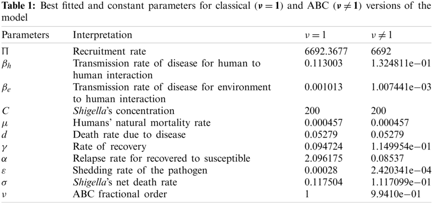
Finally, the optimal set of parameters is obtained, as shown in Tab. 1, with the least-squares approach while minimizing the absolute relative error, on average, as shown below:
where N stands for the total data value, which is 52 in this study. Moreover, real prevalent cases of the dysentery diarrhea disease, along with the classical and the ABC system’s simulations for the infected individuals, are listed in Tab. 2. In addition, Fig. 1 shows the best fit of the classical and ABC system with the real cases. The ABC system showed an average absolute relative error of 3.4284e −02, and the classical system was 3.4432e −02. Therefore, it shows that the ABC system had some advantages compared to the classical dysentery diarrhea system. In addition, the basic reproductive numbers
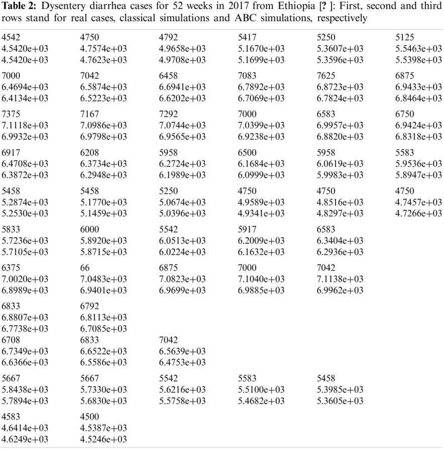
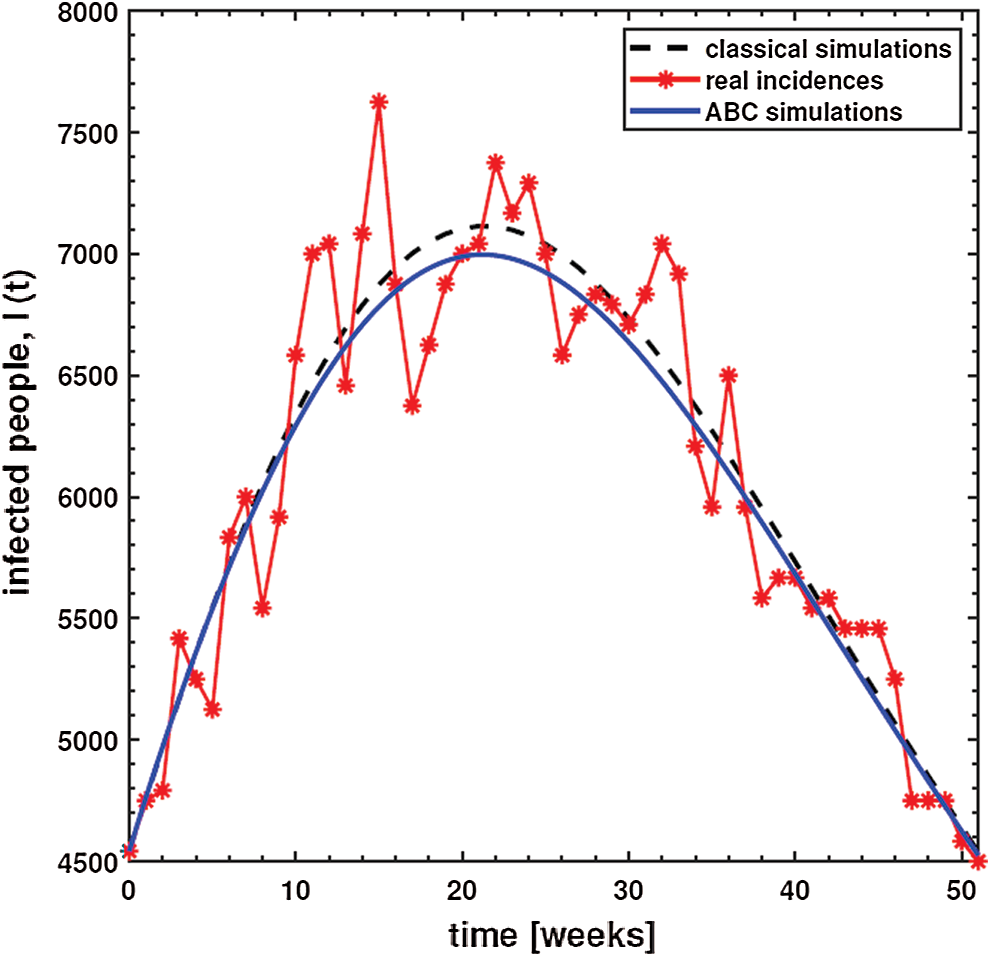
Figure 1: Plots and comparison of the real incidence cases, classical (
In this section, the concept of sensitivity analysis is used to discover the robust significance of the generic parameters present in the base reproduction number
If the dynamics follow the model (1), the analytical expressions can be used to explain the process of tracking the model’s onset at various locations. The threshold value,
where
The numerical values indicating the relative significance of R0 are given in Tab. 3. Some parameters are positive while some are negative. Parameters with positive values mean that an increase in the parameter’s values will have a major effect on the frequency of the ailment spread. On the other hand, parameters with negative values mean an increase in such parameters would decrease the effect of the disease. A representation of the values given in Tab. 3, is shown in Fig. 2.
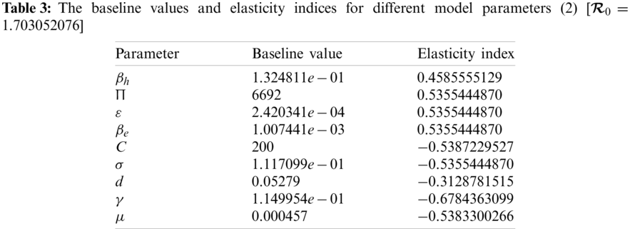
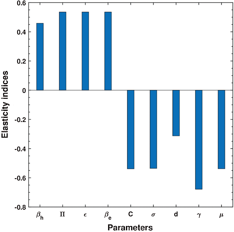
Figure 2: Elasticity indices for various parameters of
7 Simulations for the ABC Model
In this section, an algorithm is first developed to obtain the approximate solution of the ABC dysentery diarrhea model, wherein the operator uses non-local and non-singular types of the kernel. The algorithm being developed is discussed in [28], which entails the combination of the fundamental theorem of fractional calculus and two-step Lagrange type polynomial. Therefore, the fundamental theorem of fractional calculus on the Cauchy type initial value problem is given below:
This leads to:
At
With the help of interpolation polynomial, we approximate function
Eq. (24) becomes:
By solving the above integrals, we obtain the approximate solution shown below:
Hence, the proposed dysentery diarrhea model becomes:
where,
Using numerical simulations, the ABC dysentery diarrhea model (2) uses the developed algorithm shown above. Different values of the key parameters are chosen to investigate their effects on the dynamics of the disease. These parameter values are taken from Tab. 1. With simulations, we can identify important parameters that significantly affect the model’s dynamics. In order to investigate the transmission rate of dysentery due to human to human interaction (
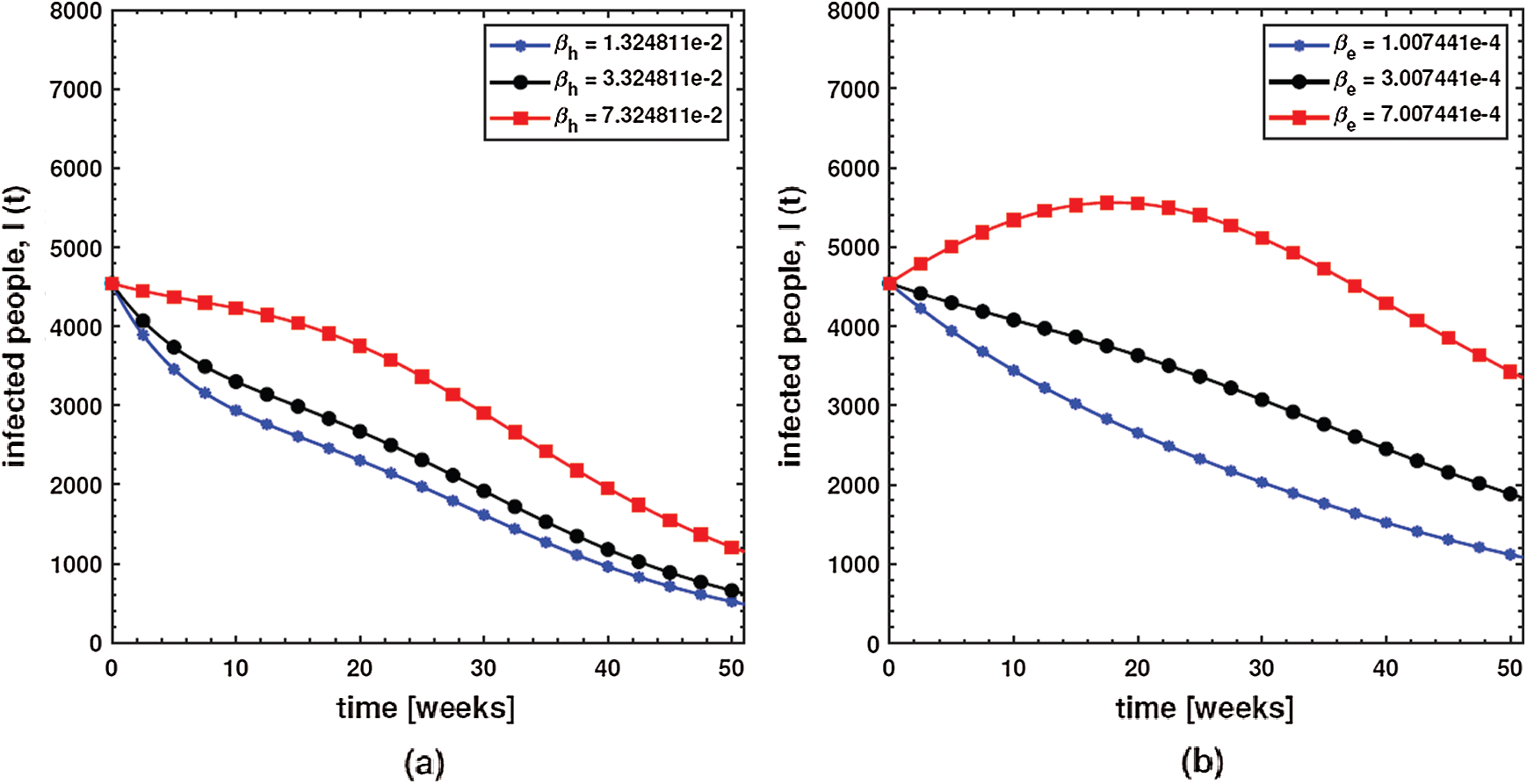
Figure 3: Behavior of diarrhea infected people with increasing values of (a) effective transmission rate of dysentery due to human to human interaction
This shows that diarrhea disease is principally due to the environment to human interaction. It means that humans must take care of their hygiene and surroundings in order to avoid the spread of dysentery. In order to investigate the effect of the concentration of Shigella pathogen (C) and the net death rate of Shigella pathogen (
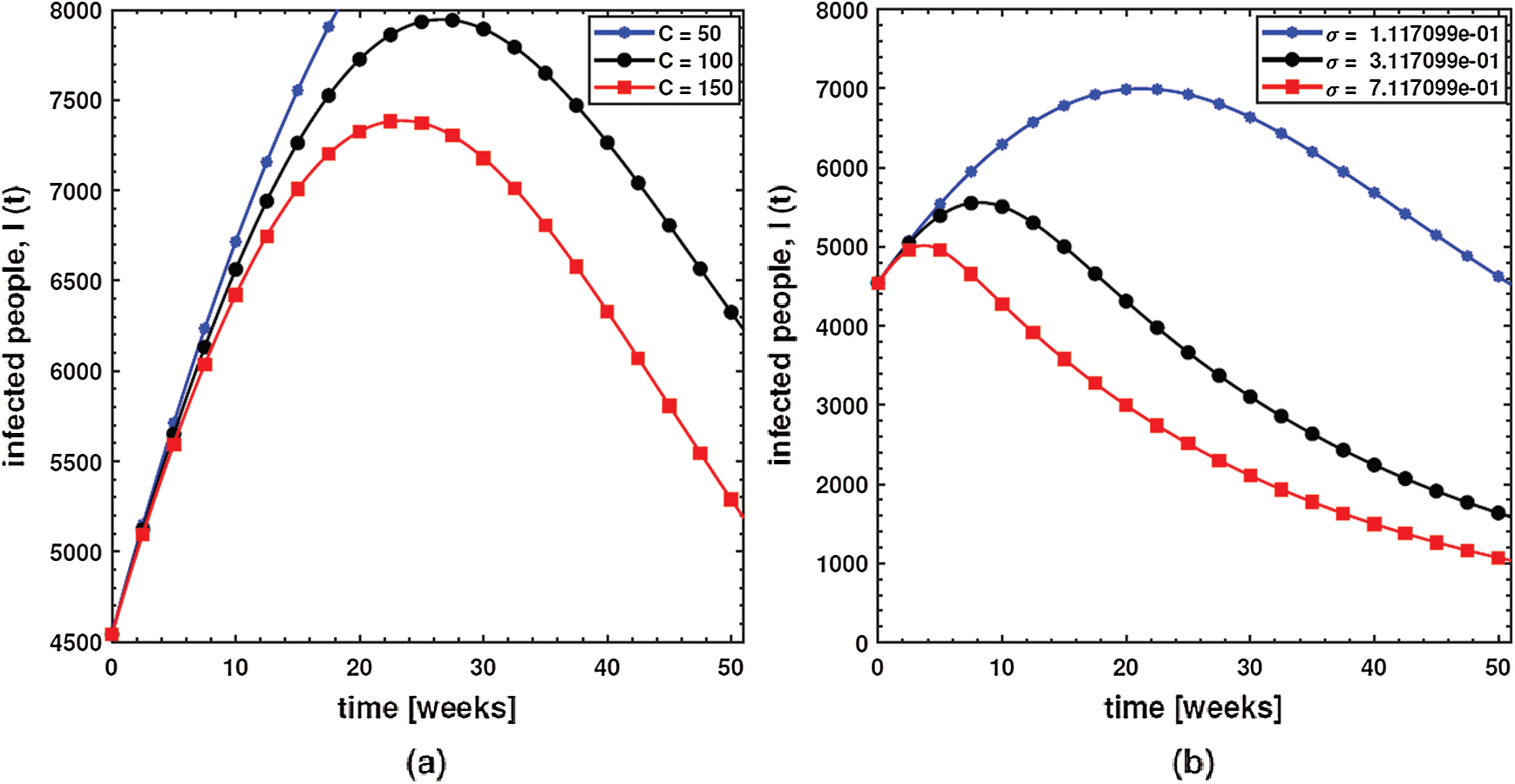
Figure 4: Behavior of diarrhea infected people with increasing values of (a) concentration of Shigella pathogen (C), and (b) net death rate of Shigella pathogen
In order to investigate the effect of the pathogen shedding rate of infected humans (
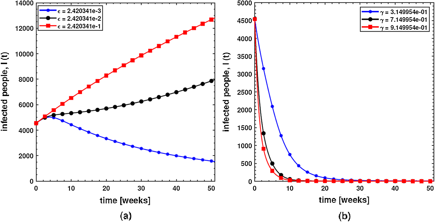
Figure 5: Behavior of diarrhea infected people with increasing values of (a) pathogen shedding rate of infected humans (
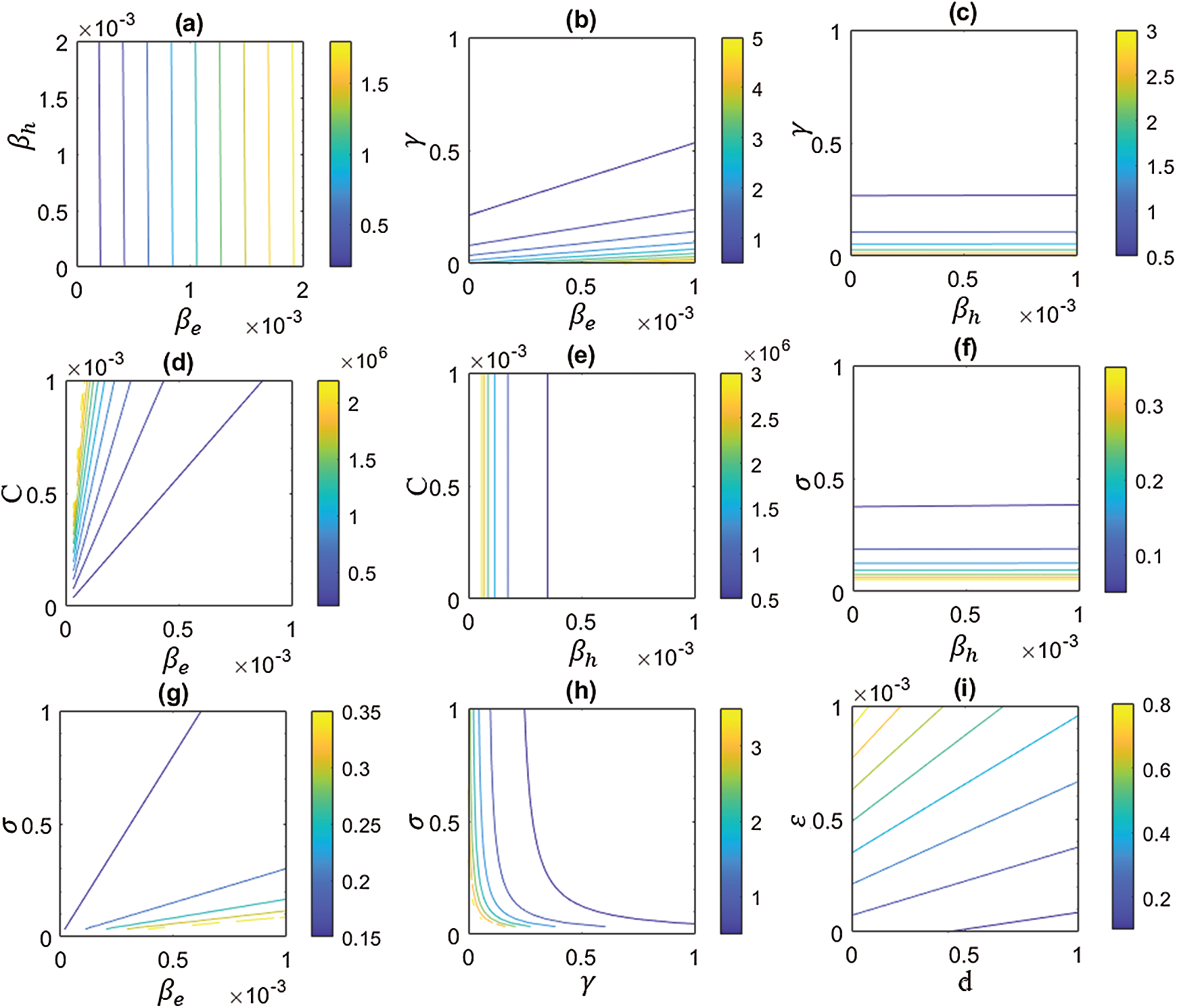
Figure 6: Behavior of basic reproductive number,
Finally, in order to investigate the effects of different parameters on the basic reproductive number,
In the present research, one of the robust non-local and non-singular fractional operator, called Atangana-Baleanu, was used to model dysentery diarrhea. The employed fractional operator was suitable for the investigation of transmission dynamics of a disease from the literature. The fractionalized order is
Furthermore, in order to shed more light on the features of the model, various numerical simulations were carried out using an effective numerical scheme. In future studies, we plan to apply the techniques used in [29–34] to understand dysentery diarrhea dynamics in greater detail. In addition, optimal control theory will be utilized to devise effective control strategies to eliminate the epidemic.
Acknowledgement: This project was funded by the Deanship of Scientific Research (DSR) at King Abdulaziz University, Jeddah, under Grant No. RG-6-135-40. The authors, therefore, gratefully acknowledge DSR technical and financial support.
Funding Statement: This research is supported by the King Abdulaziz University RG-6-135-40.
Conflicts of Interest: The authors declare that they have no conflicts of interest to report regarding the present study.
1. Rachah, A., Torres, D. F. M. (2016). Dynamics and optimal control of Ebola transmission. Mathematics in Computer Science, 10(3), 331–342. DOI 10.1007/s11786-016-0268-y. [Google Scholar] [CrossRef]
2. Ndaïrou, F., Area, I., Nieto, J. J., Silva, C. J., Torres, D. F. M. (2018). Mathematical modeling of Zika disease in pregnant women and newborns with microcephaly in Brazil. Mathematical Methods in the Applied Sciences, 41(18), 8929–8941. DOI 10.1002/mma.4702. [Google Scholar] [CrossRef]
3. Djordjevic, J., Silva, C. J., Torres, D. F. M. (2018). A stochastic SICA epidemic model for HIV transmission. Applied Mathematics Letters, 84(1), 168–175. DOI 10.1016/j.aml.2018.05.005. [Google Scholar] [CrossRef]
4. Brauer, F., Castillo-Chavez, C., Feng, Z. (2019). Mathematical models in epidemiology. USA: Springer. [Google Scholar]
5. Rao, F., Mandal, P. S., Kang, Y. (2019). Complicated endemics of an SIRS model with a generalized incidence under preventive vaccination and treatment controls. Applied Mathematical Modelling, 67, 38–61. DOI 10.1016/j.apm.2018.10.016. [Google Scholar] [CrossRef]
6. Li, L., Sun, C., Jia, J. (2018). Optimal control of a delayed SIRC epidemic model with saturated incidence rate. Optimal Control Applications and Methods, 40(2), 367–374. DOI 10.1002/oca.2482. [Google Scholar] [CrossRef]
7. Ullah, S., Khan, M. A., Gómez-Aguilar, J. F. (2019). Mathematical formulation of hepatitis B virus with optimal control analysis. Optimal Control Applications and Methods, 40(3), 529–544. DOI 10.1002/oca.2493. [Google Scholar] [CrossRef]
8. Lin, J., Xu, R., Tian, X. (2018). Global dynamics of an age-structured cholera model with both human-to-human and environment-to-human transmissions and saturation incidence. Applied Mathematical Modelling, 63, 688–708. DOI 10.1016/j.apm.2018.07.013. [Google Scholar] [CrossRef]
9. Bonyah, E., Khan, M. A., Okosun, K. O., Gómez-Aguilar, J. F. (2019). On the co-infection of dengue fever and Zika virus. Optimal Control Applications and Methods, 40, 394–421. DOI 10.1002/oca.2483. [Google Scholar] [CrossRef]
10. Ghosh, I., Tiwari, P. K., Chattopadhyay, J. (2019). Effect of active case finding on dengue control: Implications from a mathematical model. Journal of Theoretical Biology, 464(7), 50–62. DOI 10.1016/j.jtbi.2018.12.027. [Google Scholar] [CrossRef]
11. Eikenberry, S. E., Gumel, A. B. (2018). Mathematical modeling of climate change and malaria transmission dynamics: A historical review. Journal of Mathematical Biology, 77(4), 857–933. DOI 10.1007/s00285-018-1229-7. [Google Scholar] [CrossRef]
12. Kumar, D., Singh, J., Tanwar, K., Baleanu, D. (2019). A new fractional exothermic reactions model having constant heat source in porous media with power, exponential and Mittag–Leffler laws. International Journal of Heat and Mass Transfer, 138(8), 1222–1227. DOI 10.1016/j.ijheatmasstransfer.2019.04.094. [Google Scholar] [CrossRef]
13. Singh, J., Kumar, D., Baleanu, D. (2018). On the analysis of fractional diabetes model with exponential law. Advances in Difference Equations, 2018(1), 1–15. DOI 10.1186/s13662-018-1680-1. [Google Scholar] [CrossRef]
14. Kumar, D., Singh, J., Baleanu, D. (2018). A new analysis of the Fornberg–Whitham equation pertaining to a fractional derivative with Mittag–Leffler-type kernel. The European Physical Journal Plus, 133(2), 2–10. DOI 10.1140/epjp/i2018-11833-3. [Google Scholar] [CrossRef]
15. Atangana, A., Baleanu, D. (2016). New fractional derivatives with nonlocal and non-singular kernel: Theory and application to heat transfer model. Thermal Science, 20(2), 763–769. DOI 10.2298/TSCI160111018A. [Google Scholar] [CrossRef]
16. Pinto, C. M. A., Carvalho, A. R. M. (2017). A latency fractional order model for HIV dynamics. Journal of Computational and Applied Mathematics, 312(1), 240–256. DOI 10.1016/j.cam.2016.05.019. [Google Scholar] [CrossRef]
17. Jajarmi, A., Baleanu, D. (2018). A new fractional analysis on the interaction of HIV with CD4 + T-cells. Chaos, Solitons Fractals, 113(1), 221–229. DOI 10.1016/j.chaos.2018.06.009. [Google Scholar] [CrossRef]
18. Rosa, S., Torres, D. F. M. (2018). Optimal control of a fractional order epidemic model with application to human respiratory syncytial virus infection. Chaos, Solitons Fractals, 117(7–8), 142–149. DOI 10.1016/j.chaos.2018.10.021. [Google Scholar] [CrossRef]
19. Caputo, M., Fabrizio, M. (2015). A new definition of fractional derivative without singular kernel. Progress in Fractional Differentiation and Applications, 2(1), 73–85. DOI 10.12785/pfda/010201. [Google Scholar] [CrossRef]
20. Yusuf, A., Qureshi, S., Inc, M., Aliyu, A. I., Baleanu, D. et al. (2018). Two-strain epidemic model involving fractional derivative with Mittag-Leffler kernel. Chaos, 28(12), 123121. DOI 10.1063/1.5074084. [Google Scholar] [CrossRef]
21. Qureshi, S., Yusuf, A., Shaikh, A. A., Inc, M., Baleanu, D. (2019). Fractional modeling of blood ethanol concentration system with real data application. Chaos, 29, 13143. DOI 10.1063/1.5082907. [Google Scholar] [CrossRef]
22. Qureshi, S., Yusuf, A., Ali Shaikh, A., Inc, M., Baleanu, D. (2020). Mathematical modeling for adsorption process of dye removal nonlinear equation using power law and exponentially decaying kernels. Chaos: An Interdisciplinary Journal of Nonlinear Science, 30(4), 43106. DOI 10.1063/1.5121845. [Google Scholar] [CrossRef]
23. Berhe, H. W., Makinde, O. D., Theuri, D. M. (2019). Parameter estimation and sensitivity analysis of dysentery diarrhea epidemic model. Journal of Applied Mathematics, 2019(3), 1–13. DOI 10.1155/2019/8465747. [Google Scholar] [CrossRef]
24. Castillo-Chavez, C., Song, B. (2004). Dynamical models of tuberculosis and their applications. Mathematical Biosciences and Engineering, 1(2), 361–404. DOI 10.3934/mbe.2004.1.361. [Google Scholar] [CrossRef]
25. Berhe, H. W., Makinde, O. D., Theuri, D. M. (2019). Co-dynamics of measles and dysentery diarrhea diseases with optimal control and cost-effectiveness analysis. Applied Mathematics and Computation, 347(7), 903–921. DOI 10.1016/j.amc.2018.11.049. [Google Scholar] [CrossRef]
26. Berhe, H. W., Qureshi, S., Shaikh, A. A. (2020). Deterministic modeling of dysentery diarrhea epidemic under fractional Caputo differential operator via real statistical analysis. Chaos, Solitons & Fractals, 131(1), 1–13. DOI 10.1016/j.chaos.2019.109536. [Google Scholar] [CrossRef]
27. Asamoah, J. K. K., Jin, Z., Sun, G. Q., Li, M. Y. (2020). A Deterministic model for Q fever transmission dynamics within dairy cattle herds: Using sensitivity analysis and optimal controls. Computational and Mathematical Methods in Medicine, 2020(3), 1–18. DOI 10.1155/2020/6820608. [Google Scholar] [CrossRef]
28. Toufik, M., Atangana, A. (2017). New numerical approximation of fractional derivative with non-local and non-singular kernel: Application to chaotic models. The European Physical Journal Plus, 132(10), 2–16. DOI 10.1140/epjp/i2017-11717-0. [Google Scholar] [CrossRef]
29. Triet, N. A., Van Au, V., Long, L. D., Baleanu, D., Tuan, N. H. (2020). Regularization of a terminal value problem for time fractional diffusion equation. Mathematical Methods in the Applied Sciences, 43(6), 3850–3878. DOI 10.1002/mma.6159. [Google Scholar] [CrossRef]
30. Kumar, P., Qureshi, S. (2020). Laplace–Carson integral transform for exact solutions of non-integer order initial value problems with Caputo operator. Journal of Applied Mathematics and Computational Mechanics, 19(1), 57–66. DOI 10.17512/jamcm.2020.1.05. [Google Scholar] [CrossRef]
31. Tuan, N. H., Huynh, L. N., Baleanu, D., Can, N. H. (2020). On a terminal value problem for a generalization of the fractional diffusion equation with hyper-Bessel operator. Mathematical Methods in the Applied Sciences, 43(6), 2858–2882. DOI 10.1002/mma.6087. [Google Scholar] [CrossRef]
32. Qureshi, S., Chang, M., Shaikh, A. A. (2020). Analysis of series RL and RC circuits with time-invariant source using truncated M, atangana beta and conformable derivatives. Journal of Ocean Engineering and Science, 18(5), 507. DOI 10.1016/j.joes.2020.11.006. [Google Scholar] [CrossRef]
33. Bao, N. T., Baleanu, D., Minh, D., Huy, T. N. (2020). Regularity results for fractional diffusion equations involving fractional derivative with Mittag–Leffler kernel. Mathematical Methods in the Applied Sciences, 43(12), 7208–7226. DOI 10.1002/mma.6459. [Google Scholar] [CrossRef]
34. Tuan, N. H., Tri, V. V., Baleanu, D. (2020). Analysis of the fractional corona virus pandemic via deterministic modeling. Mathematical Methods in the Applied Sciences, 44(1), 1086–1102. DOI 10.1002/mma.6814. [Google Scholar] [CrossRef]
 | This work is licensed under a Creative Commons Attribution 4.0 International License, which permits unrestricted use, distribution, and reproduction in any medium, provided the original work is properly cited. |