Computer Modeling in Engineering & Sciences

DOI: 10.32604/cmes.2021.015378

ARTICLE

Variable Importance Measure System Based on Advanced Random Forest

Shufang Song1,*, Ruyang He1, Zhaoyin Shi1 and Weiya Zhang2

1School of Aeronautics, Northwestern Polytechnical University, Xi’an, 710072, China
2AECC Sichuan Gas Turbine Establishment, Mianyang, 621700, China
*Corresponding Author: Shufang Song. Email: shufangsong@nwpu.edu.cn
Received: 14 December 2020; Accepted: 17 March 2021

Nomenclature

1  Introduction

Sensitivity analysis can reflect the influence of input variables on the output response. The sensitivity analysis includes local sensitivity and global sensitivity analysis [1]. The local sensitivity can respond to the influence of input variables on the characteristics of output at the nominal value. The global sensitivity analysis, known as the importance measure analysis, can estimate the influence of input variables in the whole distribution region on the characteristics of output [2–4]. There are three kinds of importance measures: non-parametric measure, variance-based global sensitivity and moment-independent importance measure [1]. The variance-based global sensitivity is the most widely applied measure because it is generality and holistic, and it can give the contribution of group variables and the cross influence of different variables. There are plenty of methods to calculate variance-based global sensitivity indices, such as Monte Carlo (MC) simulation [5], high dimensional model representation (HDMR) [6], state-dependent parameter (SDP) procedure [7] and so on. MC simulation can estimate the approximate exact solution of total and main sensitivity indices simultaneously, but the amount of calculation is generally large, especially for high dimensional engineering problems. HDMR and SDP can calculate the main sensitivity indices by solving all order components of input-output surrogate models.

Random forest (RF) is composed by multiple decision trees (DTs), it is an ensemble learning method proposed by Breiman [8]. RF has many advantages, such as strong robustness, good tolerance to outliers and noise. RF has a wide range of application prospects, such as geographical energy [9], chemical industry [10], health insurance [11] and data science competitions. RF can not only deal with classification and regression problems but also analyze the critical measure. RF provides two kinds of importance measures: Mean Decrease Impurity (MDI) based on the Gini index and Mean Decrease Accuracy (MDA) based on Out-of-Bag (OOB) data [12]. MDI index is the average reduction of Gini impurity due to a splitting variable in the decision tree across RF [13]. MDI index is sensitive to variables with different scales of measurement and shows artificial inflation for variables with various categories. For correlated variables, the MDI index is related to the selection sequence of variables. Once a variable is selected, the impurity will be reduced by the first selected variable. It is difficult for the other correlated variables to reduce the same magnitude of impurity, so the importance of the other correlated variables will be decline. MDA index is the average reduction of prediction accuracy after randomly permuting OOB data [14,15]. Since MDA index can measure the impact of each variable on the prediction accuracy of RF model and have no biases, it has been widely used in many scientific areas. Although there are importance measures based on RF to distinguish the important features, there is no complete importance measure system to deal with nonlinearity and correlation among variables [16,17]. In addition, the similarity analysis process of MDA based on OOB data and Monte Carlo simulation of variance-based global sensitivity can be used as a breakthrough point to find their link [18]. With the help of variance-based sensitivity index system, the construction of variable importance measure system based on RF can be realized.

By comparing the procedure of estimating the total sensitivity indices and the MDA index based on OOB data, a complete VIM system is established based on advanced RF by using Kriging models, including single variable, group variables and correlated variables importance measure indices. The proposed VIM system combines the advantages of random forest and Kriging model. The VIM system can indicate the contribution of input variables to output response and rank important variables, and also give a novel way to solve variance-based global sensitivity with small samples.

This paper is organized as follows: Section 2 reviews the basic concept of variance-based global sensitivity. Section 3 reviews random forest firstly, presents MDA index and then proposes single variable, group variables and correlated variables importance measures respectively. Section 4 finds the link between MDA index and total variance-based global sensitivity index, and the relationship between VIM indices and variance-based global sensitivity indices is derived. In Section 5, several numerical and engineering examples are provided before the conclusions in Section 6.

2  Variance-Based Global Sensitivity

The variance-based global sensitivity, proposed by Sobol [19], reflects the influence of input variables in the whole distribution region on the variance of model output. The variance-based global sensitivity indices not only have strong model generality, but also can discuss the importance of group variables and quantify the interaction between input variables. ANOVA (Analysis of Variance) decomposition is the basic of variance-based global sensitivity analysis.

2.1 ANOVA Decomposition

Response function Y=g(X) exists a unique ANOVA decomposition as follows:

g(X)=g0+∑i=1ngi(Xi)+∑1≤i<j≤ngij(Xi,Xj)+…+g1…n(X1,X2,…,Xn)(1)

where n is the dimension of input variables, g0 is the expectation of g(X), g0=∫Rng(x)∏i=1n[fXi(xi)dxi], and fXi(xi) is the probability density function of variable Xi. The components in Eq. (1) are:

2.2 Variance-Based Global Sensitivity Indices

The variance of response function can be expressed as:

V=Var(Y)=∫Rng2(x)∏i=1n[fXi(xi)dxi]-g02(2)

Since the decomposition terms are orthogonal, the variance of the response function is the sum of variances of all individual decomposition terms:

where

Then the ratio of each variance component to variance of response function can reflect the variance contribution of each component, i.e., Si = Vi/V, Sij=Vij/V⋯

Si = Vi/V is the first order sensitivity index of variable Xi (also name Si as main sensitivity index), it can reflect the influence of variable Xi on the response Y. Sij = Vij/V is the second order sensitivity index, it can reflect the interaction influence of variables Xi and Xj on the response Y. The total sensitivity index SiT can be obtained by summing all the influence related to variable Xi:

According to probability theory, the variance-based global sensitivity indices can be expressed as [20]:

where X~i indicates variable vector without Xi.

2.3 Simulation of Variance-Based Global Sensitivity Indices

Due to the enormous computational load, the traditional double-loop Monte Carlo simulation is not suitable for complex engineering problems [21]. The computational procedures of single-loop Monte Carlo simulation are listed as follows:

Step 1: Randomly generate two sample matrices A and B based on the probability distribution of variables X.

Step 2: Construct sample matrix Ci, where the ith column of Ci comes from the ith column of A, and the other columns come from the corresponding columns of B.

Step 3: The main and total sensitivity indices can be expressed as follows:

Si=1N∑j=1NyAjyCij-g02Var(Y) (3)

SiT=1-1N∑j=1NyBjyCij-g02Var(Y) (4)

where yA=[yA1,…,yAN], yB=[yB1,…,yBN], yCi=[yCi1,…,yCiN] are the model outputs with the input matrices A, B and Ci respectively. The computational cost of single-loop Monte Carlo simulation is (n+2)×N.

3  Variable Importance Measure System Based on Random Forest

RF is an ensemble statistical learning method to deal with classification and regression problems [22]. Bootstrap sampling technique is firstly carried out to extract training samples from the original data, and these training samples are used to build a decision tree; the rest Out-of-Bag data are used to verify the accuracy of established decision tree.

Figure 1: Random forest

There are M established decision trees by employing Bootstrap sampling technique M times. All decision trees are used to compose a random forest (shown in Fig. 1). And the final prediction results of RF are obtained by voting in the classification model or taking the mean in the regression model [23]. And the prediction precision of RF can be expressed by mean square error square error (MSE) between predicted values and true values of OOB data.

Bootstrap technique can extract training points to build a decision tree hm (m=1,2,…,M) and the corresponding OOB data of input XOOB and output y. The decision tree hm is used to predict the forecast response ym of XOOB. The MSE of decision tree hm is εm=mean(ym-y)2. Obtain the MSEs of all decision trees εm (m=1,2,…,M), the average will be the total predicted error of RF model [24]:

MSE=1M∑m=1Mεm(5)

In order to improve the prediction precision of RF, a high-precision Kriging model is used as the model of leaf nodes in the decision tree, replacing the original average or linear regression. Next, a nonlinear discontinuous function is used to verify the prediction accuracy of Kriging model and linear regression model of decision tree.

where the input variable X is uniformly distributed on [-π, π].

A comparison of Kriging based decision tree (abbreviated as Kriging-DT) and linear regression based decision tree (abbreviated as Linear-DT) for prediction data are shown in Fig. 2. With the increase of training samples, the predicted errors of Kriging-DT and linear-DT are shown in Fig. 3. And it can be found that Kriging-DT can better approximate the original function. For the same training samples, Kriging-DT has higher prediction accuracy and faster decline rate of predicted error than Linear-DT. Kriging-DT inherits the advantages of Kriging model and has good applicability for nonlinear piecewise function.

Figure 2: Comparsion of Kriging-DT, Linear-DT and predict data with 64 training samples

Figure 3: Predicted errors of Kriging-DT and Linear-DT vs. size of training samples

There are two kinds of importance measures based on RF: Mean Decrease Impurity (MDI) based on Gini index and Mean Decrease Accuracy (MDA) based on OOB data. MDA index is widely used to rank important variables on the prediction accuracy of RF model [12].

3.1 Mean Decrease Accuracy Index of Random Forest

MDA index is the average reduction of prediction accuracy after randomly permuting OOB data. Permuting the order of variable in OOB data, the corresponding relationship between the OOB sample and output will be destroyed. The prediction accuracy will be calculated after each permutation. The MSE between the paired predictions is taken as the importance measure.

For the decision tree hm (m=1,2,…,M), the corresponding OOB input data is matrix XOOB=(XOOB1,…,XOOBi,…,XOOBn), XOOBi is the ith column of matrix XOOB. Permute the order of XOOBi, decision tree hm can obtain the new forecast response ymi. The MSE of predicted values is εmi=mean(ymi-ym)2. Obtain the influence of variable Xi in all decision trees (ε1i,ε2i,…,εMi), the average of εmi (m=1,2,…,M) is the total impact of variable Xi based on the RF model:

ηiT=1M∑m=1Mεmi(6)

The subscript m of εmi and ymi is the number of decision tree hm (m=1,2,…,M), and the superscript i of εmi and ymi indicates that the ith column of XOOB is in disorder, corresponding to the variable Xi.

Based on the procedure of MDA index, the single variable, group variables and correlated variables importance measures are expanded to establish the variable importance measure system.

3.2 Single Variable Importance Measure of Random Forest

For the decision tree hm (m=1,2,…,M), the order of OOB input data XOOB=(XOOB1,…,XOOBi,…,XOOBn) is randomly permuted expected XOOBi, that is to say, the value of variable Xi is fixed, and the values of the other variables are randomly permuted. Then the decision tree can predict the modified OOB samples to get the predicted values ym~i, the MSE of predicted values is εm~i=mean(ym~i-ym)2. Obtain the influence of variable Xi in all decision trees, the average of εm~i is the main impact of variable Xi based on the RF model:

ηi=1M∑m=1Mεm~i(7)

The superscript ~i of εm~i and ym~i indicates that the OOB data are permuted, expect for the ith columns.

3.3 Group Variable Importance Measure of Random Forest

The MDA index of group variables can be presented as follows. In the process of permuting OOB data, the values of variables Xi and Xj are fixed, and the values of the other variables are permuted. The decision tree can predict the modified OOB samples to get the predicted values ym~i,j, the MSE of predicted values is εm~i,j=mean(ym~i,j-ym)2. Obtain the influence of group variables [Xi, Xj] in all decision trees, the average of εm~i,j is the main impact of group variables [Xi, Xj] based on the RF model:

ηij=1M∑m=1Mεm~i,j(8)

The superscript ~ i, j of εm~i,j and ym~i,j indicates that the OOB data are permuted, expect for the ith and jth columns.

3.4 Correlated Variable Importance Measure of Random Forest

With the past years, several techniques based on RF are proposed to measure the importance of the correlated variables [25,26]. However, these researches directly use the independent importance measure techniques to estimate the importance of the correlated variables, which is not reasonable. Reference [27,28] divided the variance-based sensitivity indices into correlated contribution and independent contribution. Moreover, sparse grid integration (SGI) is carried out to perform importance analysis for correlated variables [29]. In the paper, the correlation of correlated variables is considered in the process of the RF importance measure. The necessary procedure of a single decision tree of the RF model for estimating the VIM consists of the following steps:

Step 1: Estimate the covariance matrix CX and mean vector μX from the original data X=(X1,…,Xi,…,Xn);

Step 2: Randomly extract the OOB data XOOB=(XOOB1,…,XOOBi,…,XOOBn) from the original data and use the other data to build the decision tree hm (m=1,2,…,M). Use the decision tree hm to predict the corresponding OOB data, and the prediction is ym;

Step 3: Split the matrix XOOB into two parts: vector XOOBi and matrix XOOB~i;

Step 4: Generate a new matrix X~i∣i and vector Xi∣~i based on XOOBi and XOOB~i, respectively. The mean vectors and covariance matrixes are different from the original μX and CX, the new ones should be used in the transformation process. For the multivariate normal distribution, μ~i∣i, μi∣~i, C~i∣i and Ci∣~i can be acquired as follows:

The mean vector μX and covariance matrix CX of X can be separated as μX=[μ~i,μi] and CX=[C~iC~i,iCi,~iCi]. The conditional mean vector and covariance matrix can be obtained by the following formulas [30]:

After obtaining the corresponding μ~i∣i, μi∣~i, C~i∣i and Ci∣~i, Nataf transform can be employed to extract normal correlation samples X~i∣i and Xi∣~i directly.

Step 5: Combine matrix X~i∣i with vector XOOBi as the new matrix XOOBnewi=(X~i∣i1,…,X~i∣ii-1,XOOBi,X~i∣ii+1,…,X~i∣in), while combine vector with the matrix XOOB~i as XOOBnew~i=(XOOB1,…,XOOBi-1,Xi∣~i,XOOBi+1,…,XOOBn);

Step 6: XOOBnewi and XOOBnew~i are passed down the decision tree and the predicted values ymi and ym~i are computed, respectively. εmi and εm~i of the correlated variables can be calculated by the following formula:

Obtain the influence of variable Xi in all decision trees, the averages of εm~i and εmi (m=1,2,…,M) are the main and total impact of variable Xi on the RF model.

The importance measure indices in correlated space and independent space are all given based on RF, which will establish the complete VIM system.

4  Link between VIM of RF and Variance-Based Global Sensitivity

The similarity analysis process of MDA index εmi based on OOB data and single-loop Monte Carlo simulation of variance-based global sensitivity can be used as a breakthrough point to find their link. The relationship between MDA index and variance-based global sensitivity can be explored firstly.

1) MDA index εmi can be decomposed as follows:

εmi=mean(ymi-ym)2=1N∑j=1N(ym,ji-ym,j)2=1N∑j=1N[(ym,ji)2+(ym,j)2-2ym,jym,ji]=1N∑j=1N(ym,ji)2+1N∑j=1N(ym,j)2-2N∑j=1Nym,jym,ji(9)

When the sample size is large, 1N∑j=1N(ym,ji)2 asymptotically equals 1N∑j=1N(ym,j)2, they are both second-order moment estimators of output response Y.

The total sensitivity index of single-loop Monte Carlo numerical simulation is:

SiT=1-1N∑j=1NyBjyCij-g02Var(Y)=1N∑j=1N(yBj)2-1N∑j=1NyBjyCijVar(Y)(10)

By comparison, it can be concluded that:

SiT=εmi2×Var(Y)(11)

Thus, the relationship between MDA index of RF importance measure and variance-based global sensitivity indices is explored. εmi can indicate the total impact of variable Xi on output performance. The larger εmi is, the larger SiT is, which means that the total contribution of variable on output performance is larger.

2) The main variance-based sensitivity index Si of single-loop Monte Carlo numerical simulation is equivalent to:

Si=1N∑j=1NyAjyCij-g02Var(Y)-1+1=1-1N∑j=1N(yAj)2-1N∑j=1NyAjyCijVar(Y)(12)

By comparison, it can be concluded that:

Si=1-εm~i2×Var(Y)(13)

Eq. (13) shows the relationship between εm~i and the main variance-based sensitivity index Si. Index εm~i can indicate the main impact of variable Xi on output performance. The larger εm~i is, the smaller Si is, which means that the main contribution of variable on output performance is smaller.

3) The relationship of variance-based sensitivity index of group variables S[i,j] and εm~i,j can be expressed as:

S[i,j]=1-εm~i,j2×Var(Y)(14)

The influence of group variables [Xi,Xj] on the variance of output S[i,j] is composed of the main sensitivity indices Si, Sj and second order sensitivity index Sij.

S[i,j]=Si+Sj+Sij(15)

Combining Eqs. (13)–(15), the second-order variance sensitivity index can be derived:

Sij=εm~i+εm~j-εm~i,j2×Var(Y)-1(16)

So far, the MDA index, single variable index and group variables index are all proposed in the independent variable space.

4) In the correlated variable space, Var(Y)≠Var(ym~i)≠Var(ymi), Eqs. (11) and (13) should be changed into the following formulas:

Si=1-εm~i-E(ym~i)2+E(ym)22×Var(Y) (17)

SiT=εmi-E(ymi)2+E(ym)22×Var(Y) (18)

Si contains the independent contribution of variable Xi and the correlated contribution of Pearson correlation coefficient, while SiT consists of the independent contribution by variable itself and interaction contribution with other variables.

5  Examples and Discussion

5.1 Numerical Example 1: Ishigami Function

Ishigami function is considered:

where Xi are uniformly distributed on the interval [-π,π], and the variables are independent. Ishigami function is a highly nonlinear function. For variable X2, the convergence trends of importance measures with the number of sample points by Monte Carlo simulation and RF are shown in Fig. 4. There are 500 decision trees in the RF model. Tabs. 1 and 2 show the VIM results of single variable and group variables respectively. The analytical results (Si(Ana), SiT(Ana) and Sij(Ana)) are also presented in Tabs. 1 and 2 for comparison.

Figure 4: The convergence trends of the important measures with sample size (a) The convergence trend of MC simulation (b) The convergence trend of RF model

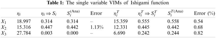
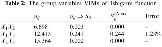
In all VIMs results tables, ηiT⇒SiT, ηi⇒Si and ηij⇒Sij mean that importance measures in this column are derived from Eqs. (11), (13) and (16), respectively.

There are 5×1020 random samples in single-loop Monte Carlo simulation to achieve the required accuracy, RF model only needs 103 samples (seen from Fig. 4). The comparison shows that RF method has faster convergence. The MDA indices of RF can get the variance-based sensitivity indices consistent with the analytical solutions (seen from Tabs. 1 and 2), which suggests the RF model provides high accuracy. For the Ishigami function, the third-order sensitivity index S123 = 0, so the relationship of the variance-based sensitivity indices is SiT=Si+∑j≠iSij, which has a good agreement with the VIM estimators.

5.2 Numerical Example 2: Linear Function with Correlated Variables

A linear model is considered [28]:

where Xi are normally distributed with μX=[0,0,0] and covariance matrix CX=[10001ρσ0ρσσ2]. Analytical solutions for the main and total sensitivity indices can be calculated as:

There are 500 decision trees and 600 samples used to analyze the importance measures. Fig. 5 shows the importance measures of the correlated input variables with different ρs. Tab. 3 shows the importance measures of independent and correlated variables cases at σ=2. Additionally, the analytical solutions are also presented for comparison.

Figure 5: The importance measures of correlated input variables at different correlation coefficients (a) Importance measures vs. correlation coefficients (b) Si-SiT vs. correlation coefficients

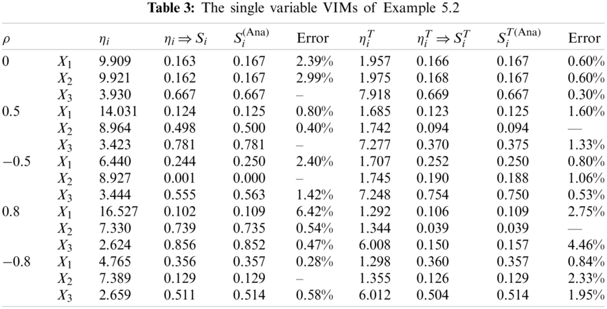
All the importance measures for correlated variables and independent ones are simulated. From the analytical results of main and total sensitivity indices, it can be found that SiT≤Si if ρ≥0 or ρ≤-2σσ2+1. The interaction sensitivity indices are all equal to zero, so Si-SiT only contain the correlated contribution by the Pearson correlation coefficients. For variable X1, the main sensitivity index S1 is equal to total indices S1T and S1-S1T=0, because of the independence of the variable X1 with other variables. For the variables X2 and X3, S2-S2T=S3-S3T, which suggests that the correlated contribution is generated from Pearson correlation coefficients.

5.3 Numerical Example 3: Nonlinear Function with Correlated Variables

Consider a nonlinear model Y = X1X3 +X2X4 [28], where X~N(μX,CX) with μX=[0,0,μ3,μ4] and covariance matrix CX=[σ12ρ12σ1σ200ρ12σ1σ2σ220000σ32ρ34σ3σ400ρ34σ3σ4σ42].

Analytical values of main and total sensitivity indices are:

where V=σ12(σ32+μ32)+σ22(σ42+μ42)+2ρ12σ1σ2(ρ34σ3σ4+μ3μ4).

Set μX=[0,0,250,400] and standard variance vector σ=[4,2,200,300]. There are 500 decision trees and 3000 samples to construct the RF model. Tab. 4 shows the VIMs results of group variables for the independent variable. The Pearson correlation coefficients are ρ12=0.3 and ρ34=-0.3. Tab. 5 shows the importance measures of single variable in the case of correlated and independent variable space.

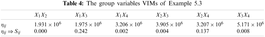
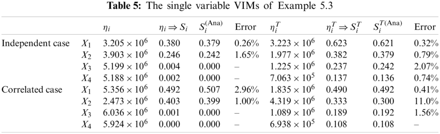
Tabs. 4 and 5 show that analytical values and numerical simulation of VIMs have good consistency. In independent variable space, the third and fourth order sensitivity indices are all equal to zero, so the relationship of important measures of single variable and group variables are also SiT=Si+∑j≠iSij.

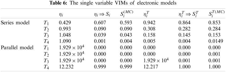
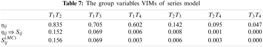
5.4 Engineering Example 4: Series and Parallel Electronic Models

Since the reliability of an electronic instrument in design stages has attracted much attention. Two simple electronic circuit models from reference [31] are used to get the VIMs. The series and parallel structures (shown in Fig. 6) are all considered in the importance measures. Each of the electronic circuit models contains four elements. The lifetime Ti independently obeys exponential distribution. The failure rate parameters are λ=[1,1/4.5,1/9,1/99], and the lifetime T of the models can be respectively expressed as:

Series model: T= min(T1,T2,T3,T4)

Parallel model: T= max(T1,T2,T3,T4)

Figure 6: The series and parallel electronic circuit structures (a) Series model (b) Parallel model

Tabs. 6 and 7 show the computational results of the importance measures by RF model, there are 500 decision trees and 15000 samples in the RF model. Due to the electronic circuit structures are discontinuous, more samples are needed to acquire the precise surrogate model and the importance measures. Additionally, the MC simulation results with 6×225 random samples are presented as approximate exact solutions Si(MC), SiT(MC) and Sij(MC) for comparison. From the comparison, the RF importance measures are also appropriate for the discontinuous model. The main sensitivity indices are almost equal to the total indices in the parallel model, while they have a significant difference in the series model (seen from Tab. 6). The second-order indices of series model are not equal to zero (seen from Tab. 7), which causes the VIMs difference between parallel model and series model.

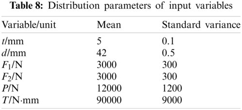
5.5 Engineering Example 5: A Cantilever Tube Model

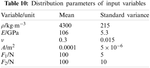
A cantilever tube model (shown in Fig. 7) is used to analyze the variable importance measures. The model is a nonlinear model with six random variables. The input variables are outer diameter d, thickness t, external forces F1, F2, P and torsion T, respectively.

Figure 7: The cantilever tube model

The tensile stress σx and the torsion stress τzx can be analyzed:

where the sectional area A, the bending moment M and the inertia moment I can be calculated by the following formula:

And the maximum stress of the cantilever can be calculated as σmax=σx 2+3τzx 2. All input variables t, d, F1, F2, P and T are normally distributed with parameters shown in Tab. 8. The Pearson correlation coefficients are ρtd=0.3 and ρF1F2=0.5. There are 500 decision trees and 7000 samples in the RF model. Tab. 9 gives the variable importance measures by RF method and the single-loop Monte Carlo simulation method. The cost of the MC method is 8×223 points for each case.

For the independent variables, the main and total sensitivity indices of input variables are very close (seen from Tab. 9), which suggests that the influence of these variables to the output response mainly come from unique variables and the interaction contribution is very small. The external force P is the most important variable in the independent space; the importance of the other input variables has a slight difference.

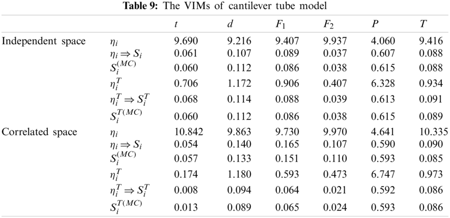
Furthermore, the importance measures are different in the correlated variable space. For the correlated input variables t, d, F1 and F2 the sensitivity indices Si>SiT, the influence on the output response mainly originates from the correlated contribution by Pearson correlation coefficients. For the input variables P and T, they are independent with other variables, so the first order indices are almost equal to total sensitivity indices. Therefore, the proposed variable RF importance measure system not only reflects the important variables but also provides useful information to identify the structure of the engineering model, which will provide useful guidance for the engineering design and optimization.

5.6 Engineering Example 6: Solar Wing Mast of Space Station

The solar wing mast of space station is a truss structure in 3D space based on triangular structure, shown in Fig. 8.

Figure 8: Solar wing mast structure [32]

The solar wing mast is made of titanium alloy. The material properties (including density ρ, Elastic modulus E, Poisson’s ration ν), external load (including dynamic load F1 and static load F2) and sectional area of truss A are random variables, the corresponding distribution parameters are listed in Tab. 10.

Software CATIA is used to establish the geometry and finite element model, and then taking the maximum stress as the output response, ABAQUS was repeatedly called to analyze the finite element model. And finally 210 samples were obtained. Random forest is used to analyze the variable importance measures, the results of VIMs are listed in Tab. 11.

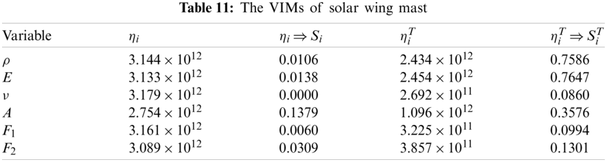
According to the results of variable importance measures, the main sensitivity index of Poisson’s ration ν is almost zero, and the total sensitivity index is also the minimum one. In order to simplify the model, the Poisson’s ration ν can be considered as a constant. The sectional area of truss A is the key design variable, since A has the largest main sensitivity to output. There is a large interaction between density ρ and Elastic modulus E, and the interaction sensitivity index can be indirectly solved SρE≈0.4623. For external load, F1 and F2 can be regarded as secondary variables. The variable importance measures can give designer reasonable suggestions to allocate optimization spaces of design variables more effectively and reduce the optimization dimension.

6  Conclusions

The Kriging regression model is used as the leaf node model of decision tree to improve the prediction accuracy of RF. The single variable, group variables and correlated variables importance measures based on RF are presented, which constitute the complete RF variable importance measure system. Additionally, a novel approach for solving variance-based global sensitivity indices is presented, and the novel meaning of these VIM indices is also introduced. The results of the numerical and engineering examples testify that the VIM indices of RF can further derive the variance sensitivity indices with higher computational efficiency compared with single-loop MC simulation.

For some incomplete probability information, such as linear correlated non-normal variables, non-linear correlated variables and discrete input-output samples and so on, the proposed importance measure analysis method has some limitations in applicability. In future work, the importance measures under incomplete probability information will be studied based on equivalent transformation or Copula function.

Authors’ Contributions: Conceptualization and methodology by Song, S. F., validation and writing by He, R. Y., examples and computation by Shi, Z. Y., examples and writing by Zhang, W. Y.

Funding Statement: The authors received no specific funding for this study.

Conflicts of Interest: The authors declare that they have no conflicts of interest to report regarding the present study.

References

 1.  Lu, Z. Z., Li, L. Y., Song, S. F., Hao, W. R. (2015). Theory and solution of importance analysis for uncertain structural systems, pp. 1–5. Beijing: Science Press (in Chinese). [Google Scholar]

 2.  Borgonovo, E. (2007). A new uncertainty importance measure. Reliability Engineering & System Safety, 92(6), 771–784. DOI 10.1016/j.ress.2006.04.015. [Google Scholar] [CrossRef]

 3.  Liu, Q., Homma, T. (2009). A new computational method of a moment-independent uncertainty importance measure. Reliability Engineering & System Safety, 94(7), 1205–1211. DOI 10.1016/j.ress.2008.10.005. [Google Scholar] [CrossRef]

 4.  Cui, L. J., Lu, Z. Z., Zhao, X. P. (2010). Moment-independent importance measure of basic random variable and its probability density evolution solution. Science China Technological Sciences, 53(4), 1138–1145. DOI 10.1007/s11431-009-0386-8. [Google Scholar] [CrossRef]

 5.  Saltelli, A., Annon, P., Auini, I. (2010). Variance based sensitivity analysis of model output: Design and estimator for the sensitivity indices. Computer Physics Communications, 181(2), 259–270. DOI 10.1016/j.cpc.2009.09.018. [Google Scholar] [CrossRef]

 6.  Ziehn, T., Tomlin, A. S. (2008). A global sensitivity study of sulphur chemistry in a premixed methane flame model using HDMR. International Journal of Chemical Kinetics, 40(11), 742–753. DOI 10.1002/kin.20367. [Google Scholar] [CrossRef]

 7.  Ratto, M., Pagano, A., Young, P. C. (2007). State dependent parameter meta-modeling and sensitivity analysis. Computer Physics Communications, 177(11), 863–876. DOI 10.1016/j.cpc.2007.07.011. [Google Scholar] [CrossRef]

 8.  Breiman, L. (2001). Random forest. Machine Learning, 45(1), 5–32. DOI 10.1023/A:1010933404324. [Google Scholar] [CrossRef]

 9.  Wang, J. H., Yan, W. Z., Wan, Z. J., Wang, Y., Lv, J. K. et al. (2020). Prediction of permeability using random forest and genetic algorithm model. Computer Modeling in Engineering & Sciences, 125(3), 1135–1157. DOI 10.32604/cmes.2020.014313. [Google Scholar] [CrossRef]

10. Yu, B., Chen, F., Chen, H. Y. (2019). NPP estimation using random forest and impact feature variable importance analysis. Journal of Spatial Science, 64(1), 173–192. DOI 10.1080/14498596.2017.1367331. [Google Scholar] [CrossRef]

11. Hallett, M. J., Fan, J. J., Su, X. G., Levine, R. A., Nunn, M. E. (2014). Random forest and variable importance rankings for correlated survival data, with applications to tooth loss. Statistical Modelling, 14(6), 523–547. DOI 10.1177/1471082X14535517. [Google Scholar] [CrossRef]

12. Cutler, A., Cutler, D. R., Stevens, J. R. (2011). Random forests. Machine Learning, 45(1), 157–176. DOI 10.1007/978-1-4419-9326-7_5. [Google Scholar] [CrossRef]

13. Loecher, M. (2020). From unbiased MDI feature importance to explainable AI for trees. https://www.researchgate.net/publication/340224035. [Google Scholar]

14. Mitchell, M. W. (2011). Bias of the random forest out-of-bag (OOB) error for certain input parameters. Open Journal of Statistics, 1(3), 205–211. DOI 10.4236/ojs.2011.13024. [Google Scholar] [CrossRef]

15. Bénard, C., Veiga, S. D., Scornet, E. (2021). MDA for random forests: inconsistency and a practical solution via the Sobol-MDA. http://www.researchgate.net/publication/349682846. [Google Scholar]

16. Zhang, X. M., Wada, T., Fujiwara, K., Kano, M. (2020). Regression and independence based variable importance measure. Computers & Chemical Engineering, 135(6), 106757. DOI 10.1016/j.compchemeng.2020.106757. [Google Scholar] [CrossRef]

17. Fisher, A., Rudin, C., Dominici, F. (2019). All models are wrong, but many are useful: Learning a variable’s importance by studying an entire cass of prediction models simultaneously. Journal of Machine Learning Research, 20(177), 1–81. http://www.jmlr.org/papers/v20/18-760.html. [Google Scholar]

18. Song, S. F., He, R. Y. (2021). Importance measure index system based on random forest. Journal of National University of Defense Technology, 43(2), 25–32. DOI 10.11887/j.cn.202102004 (in Chinese). [Google Scholar] [CrossRef]

19. Sobol, I. M. (2001). Global sensitivity indices for nonlinear mathematical models and their Monte Carlo estimates. Mathematics and Computers in Simulation, 55(1), 271–280. DOI 10.1016/S0378-4754(00)00270-6. [Google Scholar] [CrossRef]

20. Saltelli, A., Tarantola, S. (2002). On the relative importance of input factors in mathematical models: Safety assessment for nuclear waste disposal. Journal of the American Statistical Association, 97(459), 702–709. DOI 10.1198/016214502388618447. [Google Scholar] [CrossRef]

21. Saltelli, A. (2002). Sensitivity analysis for importance assessment. Risk Analysis, 22(3), 579–590. DOI 10.1111/0272-4332.00040. [Google Scholar] [CrossRef]

22. Abdulkareem, N. M., Abdulazeez, A. M. (2021). Machine learning classification based on radom forest algorithm: A review. International Journal of Science and Business, 5(2), 128–142. DOI 10.5281/zenodo.4471118. [Google Scholar] [CrossRef]

23. Athey, S., Tibshirani, J., Wager, S. (2019). Generalized random forests. The Annals of Statistics, 47(2), 1179–1203. DOI 10.1214/18-AOS1709. [Google Scholar] [CrossRef]

24. Badih, G., Pierre, M., Laurent, B. (2019). Assessing variable importance in clustering: A new method based on unsupervised binary decision trees. Computational Statistics, 34(1), 301–321. DOI 10.1007/s00180-018-0857-0. [Google Scholar] [CrossRef]

25. Behnamian, A., Banks, S., White, L., Millard, K., Pouliot, D. et al. (2019). Dimensionality deduction in the presence of highly correlated variables for Random forests: Wetland case study. IGARSS 2019–2019 IEEE International Geosciences and Remote Sensing Symposium, pp. 9839–9842, Yokohama, Japan. [Google Scholar]

26. Gazzola, G., Jeong, M. K. (2019). Dependence-biased clustering for variable selection with random forests. Pattern Recognition, 96, 106980. DOI 10.1016/j.patcog.2019.106980. [Google Scholar] [CrossRef]

27. Mara, T. A., Tarantola, S. (2012). Variance-based sensitivity indices for models with dependent inputs. Reliability Engineering & System Safety, 107(11), 115–121. DOI 10.1016/j.ress.2011.08.008. [Google Scholar] [CrossRef]

28. Kucherenko, S., Tarantola, S., Annoni, P. (2012). Estimation of global sensitivity indices for models with dependent variables. Computer Physics Communications, 183(4), 937–946. DOI 10.1016/j.cpc.2011.12.020. [Google Scholar] [CrossRef]

29. Li, L. Y., Lu, Z. Z. (2013). Importance analysis for models with correlated variables and its sparse grid solution. Reliability Engineering & System Safety, 119, 207–217. DOI 10.1016/j.ress.2013.06.036. [Google Scholar] [CrossRef]

30. He, X. Q. (2008). Multivariate statistical analysis, pp. 9–14. Beijing: Renmin University Press (in Chinese). [Google Scholar]

31. Song, S. F., Wang, L. (2017). Modified GMDH-NN algorithm and its application for global sensitivity analysis. Journal of Computational Physics, 348(1), 534–548. DOI 10.1016/j.jcp.2017.07.027. [Google Scholar] [CrossRef]

32. He, R. Y. (2020). Variable importance measures based on surrogate model, pp. 66–69. Xi’an: Northwestern Polytechnical University (in Chinese). [Google Scholar]

This work is licensed under a Creative Commons Attribution 4.0 International License, which permits unrestricted use, distribution, and reproduction in any medium, provided the original work is properly cited.