Computer Modeling in Engineering & Sciences

DOI: 10.32604/cmes.2021.014847

ARTICLE

A Numerical Model for Simulating Two-Phase Flow with Adaptive Mesh Refinement

Yunxing Zhang, Shan Ma, Kangping Liao and Wenyang Duan*

Harbin Engineering University, Harbin, 150001, China
*Corresponding Author: Wenyang Duan. Email: duanwenyang_heu@hotmail.com
Received: 03 November 2020; Accepted: 11 March 2021

1  Introduction

Two-phase flow is very important as it is common in many engineering fields, ranging from naval hydrodynamics, geophysics to ocean engineering. The experimental study is a widely used approach for analyzing physical problems. However, due to the existence of small-scale structures and violent velocity change, experimental measurements on violent two-phase flow problems could be extremely difficult or even impossible. With the improvement of hardware and numerical algorithms, numerical simulation could be a powerful alternative for predicting the behaviors of these problems. However, there still exist many difficulties in numerical simulating two-phase flow.

Among the difficulties, the computational cost could be one of the major challenges in Computational Fluid Dynamics (CFD). Traditionally, a fixed structured grid is usually adopted for simulating two-phase flow problems. One of the remarkable features of this grid is that mesh refinement needs to be applied in priority on the range of all the caring regions, which is inefficient or even impossible when the caring regions are unpredictable. Adaptive Mesh Refinement (AMR) grid was proposed by Berger et al. [1] which allows refining certain regions of the zone during the simulation to reduce the computational effort required. Since then, the AMR grid was widely used to simulate various kinds of flows.

For most of the research with AMR, single-phase flow is considered. As the method was proposed for hyperbolic partial differential equations, a natural implementation of AMR is the solution of the Euler equation [2,3]. Moreover, it was combined with the immersed boundary method for fluid-structure interaction problems of solid bodies [4,5] or flexible bodies [6,7] to combine the advantages of the two methods.

Research that applying AMR in two-phase flow is also numerous, relevant research can be found in surface-tension-driven interfacial flows such as bubbles [8–10], bubble/jet interact with bodies [11], and wave breaking or wave-body interactions [12–15]. However, it is still hard work to develop such a model. The difficulties include the large-density ratio and complex interface topology in two-phase flow, as well as the treatment of coarse-fine interface in the AMR grid where conservation is hard to preserve.

The objective of this paper is to develop a 3D numerical model for simulating two-phase flow with AMR. The model is the foundation of future work for wave-body interactions in the ship and ocean engineering field. To develop such a model, the difficulties discussed above should be considered. The first one is the complex interface topology, or in other words, to capture the gas-water interface accurately. For this problem, widely used methods include the front tracking method [16], the level set method [17], and the VOF method [18]. Among the methods, the accuracy and robustness of the VOF method were widely demonstrated [19]. For simplicity, the VOF method is adopted in this model. However, other methods can also be applied in this model as alternatives.

Large density ratios usually exist in two-phase flow, such as in bubble flow in which the density ratio could reach 106. This large ratio can result in numerical instability which may come from gas velocities being mixed with liquid densities [10,20]. It was demonstrated that a mass-momentum consistent transport can alleviate the instability [10,20–23]. The influence of high-density ratio on inconsistent transport of mass and momentum is complex. A detailed comparison between consistent and inconsistent transport of mass and momentum for high-density-ratio flows can be found in [21,22]. In fact, both inconsistent and consistent schemes can be found in two-phase flow simulations. With inconsistent transport schemes, acceptable results were observed for wave-body interactions [15] and bubble evolution [9]. Besides, consistent schemes were successfully applied to simulate wave energy converters [24–26] and water entry [27] problems. Consider the complexity of the numerical schemes and the objective of the solver, inconsistent transport of mass and momentum is adopted at present. Therefore, to validate the feasibility of inconsistent transport schemes is also one of the objectives of the paper.

A 3D numerical model for simulating two-phase flow with AMR is developed in this paper. The VOF method is adopted to capture the gas-water interface accurately. A coarse-fine interface treatment method for two-phase flow is developed to preserve the flux conservation at the coarse-fine interfaces. An inconsistent transport scheme is adopted for the advection of mass and momentum. The work is based on Zhang et al. [15] in which a 2D model is developed. The paper is organized as follows: The governing equations, single grid solver, and the AMR grid are introduced in Section 2, with special attention paid to discretization schemes and the coarse-fine interface treatment methods. The validations of the numerical model are given in Section 3 with selected cases. The accuracy of VOF on the AMR grid and the entire model is demonstrated. Further validation of the model is presented in Section 4 with more serious problems to show the ability of the model on simulating wave breaking problems. Finally, the conclusions are drawn in Section 5.

2  Numerical Methods

2.1 Governing Equations

The single fluid formulation for multiphase flow is adopted in this model [28]. The viscous incompressible two-phase flow is considered as a fluid with spatially and temporally varying density and viscosity. The fluid is governed by the continuity equation and the Navier-Stokes equations, which in the non-conservative form are:

∇⋅u=0∂u∂t+∇⋅uu=−1ρ∇p+1ρ∇⋅[ μ(∇u+∇uT) ]+f (1)

in which u=(u,v,w) is the velocity of the fluid, p is the pressure, ρ and μ are the density and the dynamic viscosity coefficient, f stands for the body forces such as the gravitational force. The Eq. (1) is applied to a fixed Eulerian space with x=(x,y,z) to be the Eulerian coordinates.

The VOF method is utilized to capture the free surface. In the method, a scalar function φ is defined to represent the water phase. The value of φ for a cell is between 0 and 1 which denotes the fraction volume of the water phase within the cell. The evolution equation of φ is:

∂φ∂t+∇⋅(uφ)=0 (2)

Appropriate initial and boundary conditions for Eqs. (1) and (2) are necessary. For all the simulations, water is initially at rest, and velocities are set to zero at the initial stage. The initial values of φ are defined with the topology of the water phase. All the boundaries are defined as walls, so the Dirichlet condition is used for the velocities and the Neumann condition is adopted for the pressure.

2.2 Single Grid Solver

In this section, the numerical methods on a single grid are introduced. For simplicity, the discretization schemes of the spatial derivatives are given in the 2D form. There is no extra difficulty for their extension to 3D.

2.2.1 Time Integration

The incompressible version of the projection method proposed by Xiao [29] is utilized for the time integration. The Navier–Stokes equation in Eq. (1) is split into three steps: one advection step and two non-advection steps.

Advection step

u∗−unΔt+∇⋅unun=0 (3)

Non-advection Step I

u∗∗−u∗Δt=1ρn+1∇⋅[μn+1(∇u∗+∇u∗T)]+f∗∗ (4)

Non-advection Step II

un+1−u∗∗Δt=−1ρn+1∇⋅pn+1 (5)

Here the corner mark n, n+1, *, and ** indicate the values of corresponding quantities at the current time step, the next time step, and the two predicted values between the two steps. This procedure was demonstrated to yield the first-order accuracy in time integration [29].

By applying the continuity equation in Eq. (1) to the Eq. (5), the following Pressure Poisson Equation (PPE) is obtained:

∇⋅(1ρ∇pn+1)=1Δt∇⋅u∗∗ (6)

The pressure is calculated by solving the equation after non-advection Step I and followed by non-advection Step II.

To ensure the temporal stability of the explicit projection method in the model, the time step Δt is defined concerning the convective effects. The time step Δt is determined with the following Courant–Friedrichs–Lewy (CFL) condition with C no more than 0.5 adopted for all the simulations.

Δt≤min(CΔxmax‖u‖∞,CΔymax‖v‖∞) (7)

2.2.2 Discretization of the Spatial Derivatives

The Finite Difference Method (FDM) on the Cartesian grid with a staggered arrangement of variables is adopted. A 2D case is illustrated in Fig. 1. The velocities are located on the cell side and scalars such as pressure and density are located on the cell center.

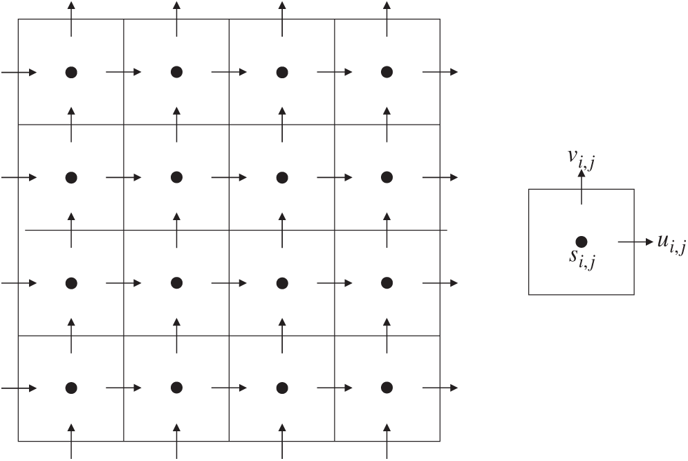
Figure 1: The staggered arrangement of the variables (s indicates for scalars)

For the discretization of the advection step (Eq. (3)), the upwind schemes are usually adopted to enhance the robustness of the code. A conservative discretization scheme is adopted as follow:

∂ui,j∂t=−(ui,j+ui+1,j)u˜i+1/2,j−(ui,j+ui−1,j)u˜i−1/2,j2Δx−(vi,j+vi+1,j)u˜i,j+1/2−(vi,j−1+vi+1,j−1)u˜i,j−1/22Δy (8)

∂vi,j∂t=−(ui,j+ui,j+1)v˜i+1/2,j−(ui−1,j+ui−1,j+1)v˜i−1/2,j2Δx−(vi,j+vi,j+1)v˜i,j+1/2−(vi,j+vi,j−1)v˜i,j−1/22Δy (9)

The values of u˜ and v˜ at the cell edge (i±1/2,j or i,j±1/2) are calculated with the QUICK scheme [30] combined with Van Leer TVD limiter [31]. The interpolation stencil is determined based on the sign of the coefficient before it.

The central difference method is adopted for all the spatial derivatives in Eqs. (4)–(6). For non-advection step I (Eq. (4)), the discretization for the horizontal velocity u and the vertical velocity v is:

∂ui,j∂t=fxi,j+1ρi+1/2,j{2Δx[μi+1,jui+1,j−ui,jΔx−μi,jui,j−ui−1,jΔx]+1Δy[μi+1/2,j+1/2(ui,j+1−ui,jΔy+vi+1,j−vi,jΔx)]−1Δy[μi+1/2,j−1/2(ui,j−ui,j−1Δy+vi+1,j−1−vi,j−1Δx)]} (10)

∂vi,j∂t=fyi,j+1ρi,j+1/2{1Δx[μi+1/2,j+1/2(vi+1,j−vi,jΔx+ui,j+1−ui,jΔy)]−1Δx[μi−1/2,j+1/2(vi,j−vi−1,jΔx+ui−1,j+1−ui−1,jΔy)]+2Δy[μi,j+1vi,j+1−vi,jΔy−μi,jvi,j−vi,j−1Δy]} (11)

The discretization of Eq. (5) is easy to derive and is neglected here. The discretization of PPE (Eq. (6)) is as follows:

1Δt(ui,j−ui−1,jΔx+vi,j−vi,j−1Δy)=pi+1,j(1Δx21ρi+1/2,j)+pi−1,j(1Δx21ρi−1/2,j)+pi,j+1(1Δy21ρi,j+1/2)+pi,j−1(1Δy21ρi,j−1/2)−pi,j[1Δx2(1ρi+1/2,j+1ρi−1/2,j)+1Δy2(1ρi,j+1/2+1ρi,j−1/2)] (12)

2.2.3 VOF Equation

For the solution of Eq. (2), PLIC is utilized to reconstruct the interface [32]. The Lagrangian advection scheme is adopted to propagate the interfaces within the cells [33].

With the φ of a cell determined, the density and dynamic viscosity coefficient at the cell center are defined with:

ρi,j=φi,j⋅ρwater+(1−φi,j)⋅ρgas (13a)

μi,j=φi,j⋅μwater+(1−φi,j)⋅μgas (13b)

In the discretizations of the two non-advection steps and the PPE equation (Eqs. (10)–(12)), the densities and dynamic viscosity coefficients at the cell edges and corners are necessary. If the viscous term in the Navier–Stokes equations is treated implicitly, the harmonic averaging method is suggested [10]. As the viscous term is treated explicitly in this model, the simple average method is adopted for simplicity:

si+1/2,j=(si,j+si+1,j)/2 (14a)

si+1/2,j+1/2=(si,j+si+1,j+si,j+1+si+1,j+1)/4 (14b)

where s stands for the density and dynamic viscosity coefficient.

2.3 AMR Grid

2.3.1 AMR Grid and Data Structure

As mentioned before, the AMR grid is employed in this model. The computation domain is defined as a quadtree (2D) or octree (3D) structure with all the nodes of the tree to indicate a grid block with the same grid number (see Figs. 2 and 3 for the grid and the corresponding data structure). During the simulation, the grid is allowed to refine/coarsen certain blocks based on the defined strategy. It is noted that the refinement level is not allowed to jump more than one at any location during the refining/coarsen process. In this paper, the open-source library Paramesh is utilized to manage the grid [34].

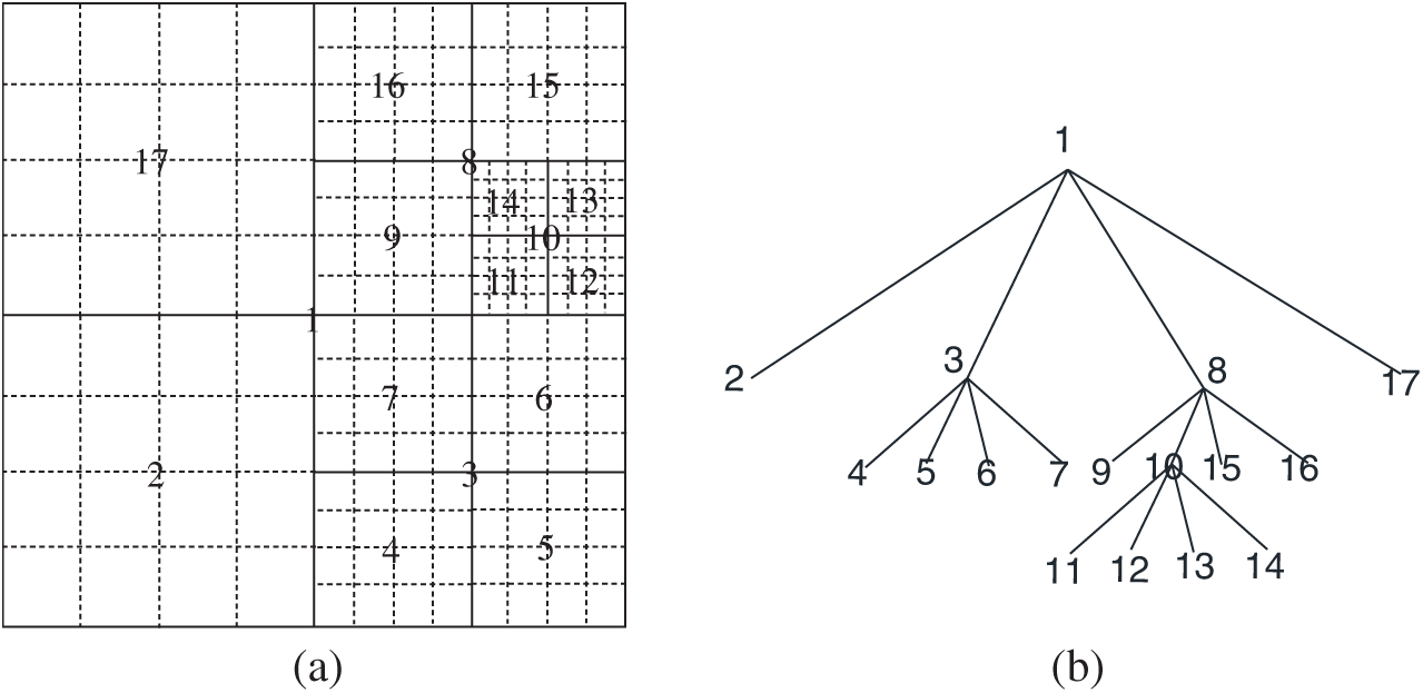
Figure 2: (a) AMR grid and (b) the corresponding data structure in 2D

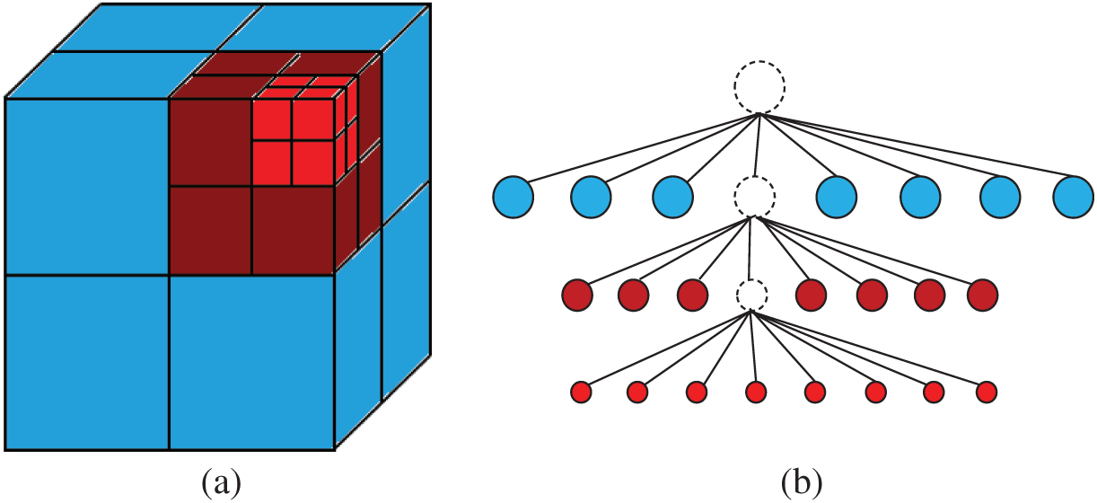
Figure 3: (a) AMR grid and (b) the corresponding data structure in 3D

A fixed time step strategy is adopted due to the incompressibility of the fluid. The single grid solver is applied on all the grid blocks without too many changes, except for the interpolation between blocks to provide boundary conditions.

2.3.2 Interpolation and Refining/Coarsen Operators

After each operation (advection, diffusion, and pressure correction) within each time step, interpolations are necessary as the grid blocks need ghost cells at their boundaries to complete the discretization stencils. Two layers of ghost cells are used for each block. Take the grid in Fig. 2 as an example, for the blocks at the same level (such as 9 and 16), the direct injection method is used. For the blocks whose ghost cell values are provided by a finer grid block (such as 17 provided by 9 and 16), the simple average method is used to preserve the accuracy as well as conservation. For the blocks whose ghost cell values are provided by a coarser grid block (such as 7 or 4 provided by 2), the algorithm is a little bit complex and we will interpret it in detail.

Due to the staggered arrangements of the variables, the interpolations for variables u and v are different. As shown in Fig. 4, ui−1,j, ui−2,j, vi−1,j and vi,j are needed for the fine grid. In this model, the bi-quadratic interpolation is adopted to achieve 2nd-order accuracy. The expressions are:

ui−2,j=(5UI,J+1+30UI,J−2UI,J−1)/32ui−1,j=(ui−2,j+ui,j)/2vi−1,j=(VI,J+7VI+1,J−vi+1,j)/7vi,j=(8VI+1,J+10vi+1,j−3vi+2,j)/15 (15)

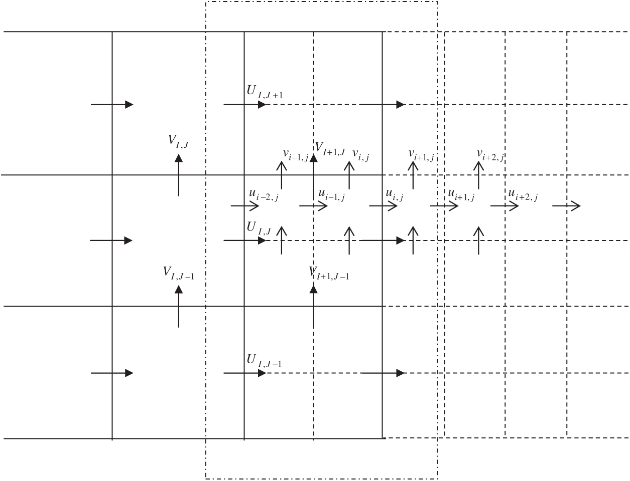
Figure 4: Interpolations between coarse grid (solid lines with variables in the upper case) and fine grid (dashed lines with variables in the lower case), interpolation zone indicated with a box in the dash-dotted line

Other interpolations can be categorized into the expressions above. The interpolations in 3D are similar.

A refining/de-refining process is conducted based on the distance of a grid block from the free surface at the end of each time step. During the process, the divergence-free condition must be preserved. Here, the face averaging method is adopted for the de-refining process as it is a simple way to preserve the divergence of the velocity field on a staggered grid as well as global 2nd-order accuracy. For the refining process, the method proposed by Tóth et al. [35] in which a prolongation operator that can preserve the divergence and curl is employed.

2.3.3 Coarse-Fine Interface Treatment

A careful treatment of the coarse-fine interface is necessary during the solution process. Due to the staggered grid, velocities at the interface will share the same face for the coarse and fine grid as shown in Fig. 5. Flux conservation is necessary at the interface. The velocity on the finer grid is considered to be more accurate so a simple average is performed after each operation (advection step, diffusion step, and pressure correction step), which has the form of UI,JΔY=(ui,j+ui,j−1)Δy. However, as the divergence-free condition is already fulfilled after the pressure correction step, the condition may no longer be preserved if an additional flux conservation operation is performed at the end of each time step.

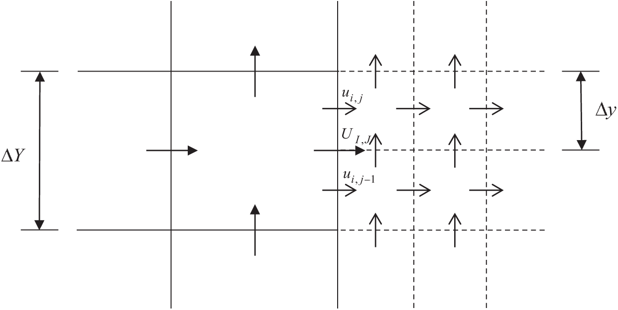
Figure 5: Flux conservation at the coarse-fine interface

A simple method to avoid the situation is to force the velocities to satisfy the flux conservation condition after the pressure correction step automatically. A pressure boundary condition method is proposed by Vanella et al. [4] for single-phase flow. The method could be extended to two-phase flow with the consideration of density variation. During the iterative solution of PPE, the gradient of the pressure normal to the coarse-fine interface is forced to satisfy the following equation:

1ρ∂pcoarse∂x|I,JΔY=1ρ∂pfine∂x|i,jΔy+1ρ∂pfine∂x|i,j−1Δy (16)

Then the flux conservation condition will be automatically satisfied.

2.4 Algorithm

The complete algorithm of the model is as follows:

1.    Initialize the flow field with the initial topology of the water phase (φn), the velocity field (un) and the pressure field (pn).

2.    Calculate the position of the interface at the new time step to obtain φn+1 by advecting the VOF equation (Eq. (2)).

3.    Obtaining the density and dynamic viscosity coefficient of the cell (ρn+1, μn+1) with φn+1 (Eq (13)).

4.    Compute the provisional velocity field u∗ using Eq. (3).

5.    Compute the provisional velocity field u∗∗ using Eq. (4).

6.    Calculate the pressure field pn+1 using Eq. (6).

7.    Compute the velocity field un+1 using Eq. (5).

8.    Compute the distance from free surface for each grid block, refine/de-refine the blocks under the defined strategy.

9.    Proceed to Step (2) for the next time step.

3  Validations

In this section, three selected benchmark cases are carried out for the validation of the model. Shear flow tests are conducted to validate the extension of the VOF method to the AMR grid. A linear sloshing case is considered to check the accuracy of the model. A nonlinear sloshing problem is simulated to validate the accuracy of the model as well as discuss the efficiency with the AMR grid.

3.1 2D/3D Shear Flow Test

The shear flow test is a widely used benchmark to validate the VOF method [36]. In this problem, an initial scalar field evolves under a given velocity field. The forms of the velocity field are:

2D u(x,y)=sin⁡(πx)cos⁡(πy)v(x,y)=−cos⁡(πx)sin⁡(πy) (17a)

3D u(x,y,z,t)=2sin2⁡(πx)sin⁡(2πy)sin⁡(2πz)cos⁡(πt/T)v(x,y,z,t)=−sin⁡(2πx)sin2⁡(πy)sin⁡(2πz)cos⁡(πt/T)w(x,y,z,t)=−sin⁡(2πx)sin⁡(2πy)sin2⁡(πz)cos⁡(πt/T) (17b)

The zone scale is 1.0 for both 2D and 3D on all the dimensions. The initial shape of the scalar field is given as a circle in 2D and a sphere in 3D. So the corresponding volume fraction is set as:

2D φ={1(x−0.5)2+(y−0.25)2<0.150else (18a)

3D φ={1(x−0.35)2+(y−0.35)2+(z−0.35)2<0.150else (18b)

A 4-level AMR grid is used with the CFL number set to be 0.1 for all the simulations. The minimum scale of the grid is set as 1/128. The results at selected moments are shown in Figs. 6 and 7. For the 2D case, at time t = 5 s (Fig. 6a), discontinuity of the scalar field is observed. It is due to the incorrect normal direction and can be alleviated with a finer mesh. At time t = 10 s (Fig. 6b), the scalar field evolves back to a circle. For the 3D case, the sphere evolves to be disk type at t = 0.5T (Fig. 7a) and then evolves back to a sphere at t = T (Fig. 7b). The results are acceptable considering the results of previous works [13,36].

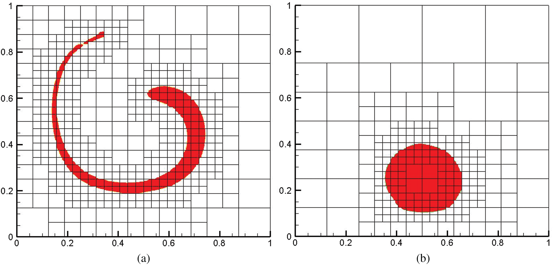
Figure 6: 2D scalar fields at selected moments (velocity field change sign symbol at t = 5 s): (a) t = 5 s; (b) t = 10 s

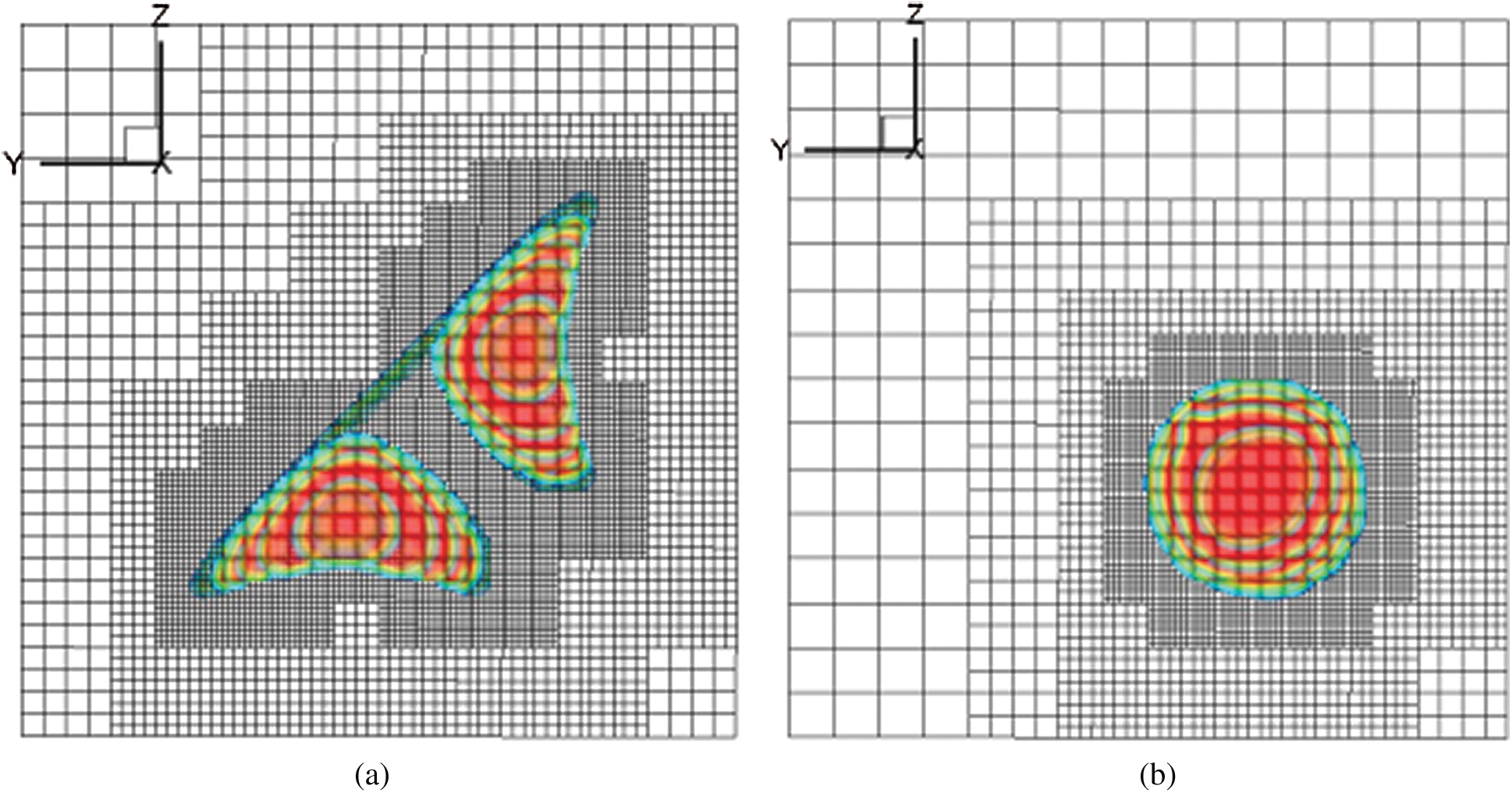
Figure 7: 3D scalar fields at selected moments (T = 3 s): (a) t = 0.5 T; (b) t = T

3.2 2D Linear Free Sloshing with Viscous Effects

2D linear free sloshing is considered to validate the accuracy of the model. In this problem, a tank is filled with water and gas and the initial wave profile is given. The liquid is initially at rest and evolves submitted to the gravity force. An illustration of the problem is presented in Fig. 8.

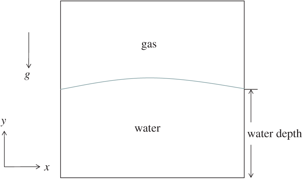
Figure 8: Illustration of the linear free sloshing problem

When the wave amplitude is small, a linear analytic solution for 2D viscous waves in a rectangular tank was derived by Wu et al. [37]. For the initial wave profile to be:

η0=acos⁡k(x+W/2) (19)

where W is the width of the tank, a is the initial wave amplitude and k is the wave number with k=2π/W. When the condition that κ=g/ν2k3>0.5814122 is fulfilled where v is the kinematic viscosity of the liquid and g is the gravity acceleration, the analytical solution for free surface profile deformation can be expressed in the following form:

η(t)η0=1−2κℜ(∑i=12Ai{−γie(−1+γi2)νk2t[1+erf(γikνt)]+γi+erf(kνt)}1−γi2) (20)

in which ℜ means the real part of the complex number, γ1 and γ2 are any non-conjugate roots of the four possible roots of the following equation:

(x2+1)2−4x+κ=0 (21)

Here the width of the tank, the water depth, and the initial wave amplitude are set as 1.0 m, 0.5 m, and 0.01 m, respectively. A 4-level AMR grid is adopted for this case. The grids are uniform around the interface in both directions with the spacing of 1/128 m. A constant time step of 0.00001 s is used for all the simulations. Reynolds numbers of 20 and 200 are considered here to validate the model and both cases run up to 10 s. The results are shown in Fig. 9 with a comparison to the analytic solution and good agreement is obtained. It is observed that the decrease of wave amplitude for Re to be 20 is very fast, due to the large viscosity.

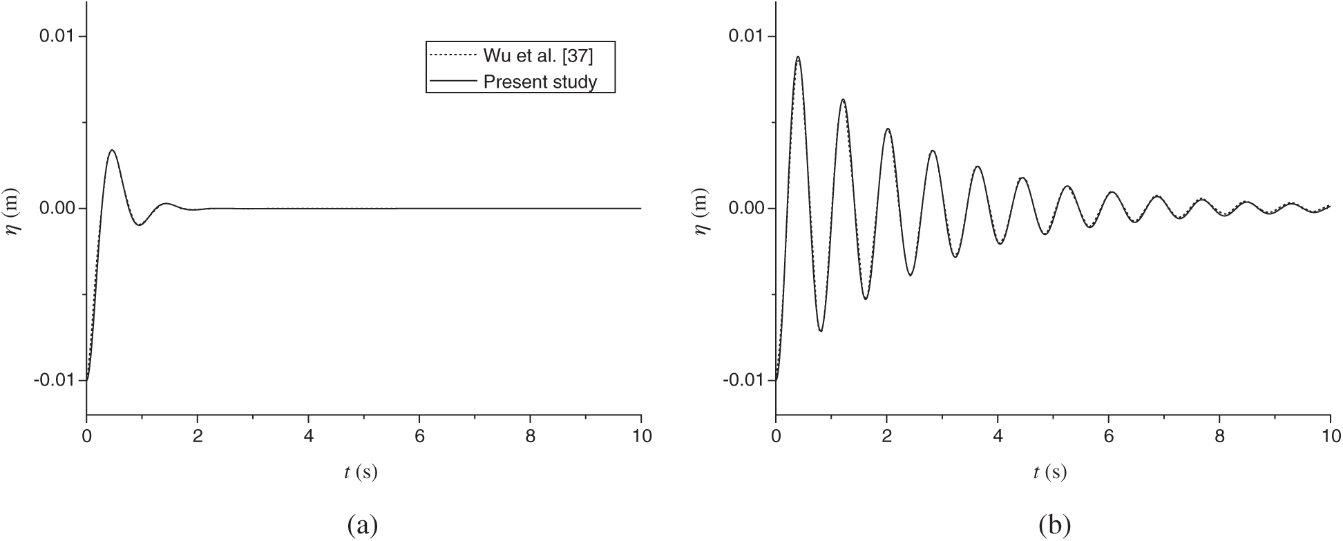
Figure 9: Time histories of the wave amplitudes for (a) Re = 20; (b) Re = 200. (Here Re=hgh/ν)

The spatial accuracy of the model is measured with the problem. The L2 and L∞ norm errors of the solution of free surface height are shown in Fig. 10. The solution on the 256×256 grid is defined as the reference solution. As shown in Figs. 10a and 10b, the L2 norm error is nearly 2nd-order while the L∞ norm error is between 1st-order and 2nd-order. The error should come from the smear near the free surface in the discretization (Eqs. (13) and (14)).

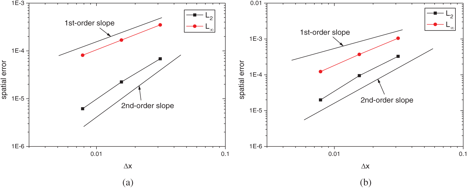
Figure 10: Variations of the norm errors of the free surface height with different grid spacing: (a) Re = 20; (b) Re = 200

3.3 2D Nonlinear Sloshing under Surge Motion

A 2D nonlinear sloshing resonance problem is considered with this model. In this problem, a partially filled tank submitted to the gravity force and an external horizontal force is simulated. The computational model with corresponding parameters consistent with Liu et al.’s [38] experiment is shown in Fig. 11. When the frequency of the exciting force is close to the natural frequency of a tank, resonance will occur. For a 2D case, the natural frequency can be obtained with ωn=gkntan⁡h(knd) where d is the water depth and kn = nπ/W, here W is the width of the tank [39]. The width of the tank and the water depth are 0.57 m and 0.15 m, so the lowest natural frequency is ωn=6.0578 s−1. The water in the tank is at rest at t = 0 s. Under the external force, the movement of the tank follows x=−asin⁡ωt in which the amplitude a is 0.005 m and ω=ωn. So that resonance will occur after some time.

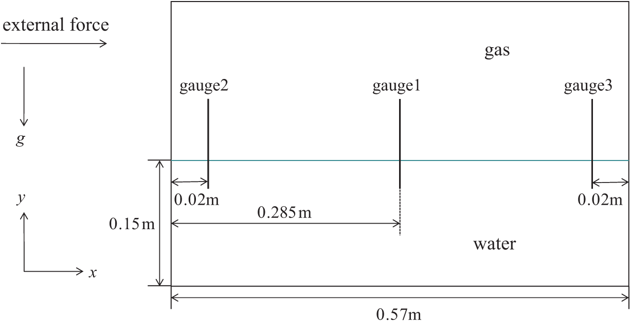
Figure 11: Computational model of 2D nonlinear sloshing

A 4-level AMR grid is adopted with the finest grid to be 0.0045 m in both directions. A constant time step of 0.001 s is used. Time histories of the free surface height at the three gauges for the time before 6.7 s are shown in Fig. 12. The linear analytic solution is also given. The results agree very well with the experimental data of [38]. While the linear analytic solution gives an acceptable prediction only for the time before about 3 s. Then it fails to predict the behavior due to the nonlinearity.

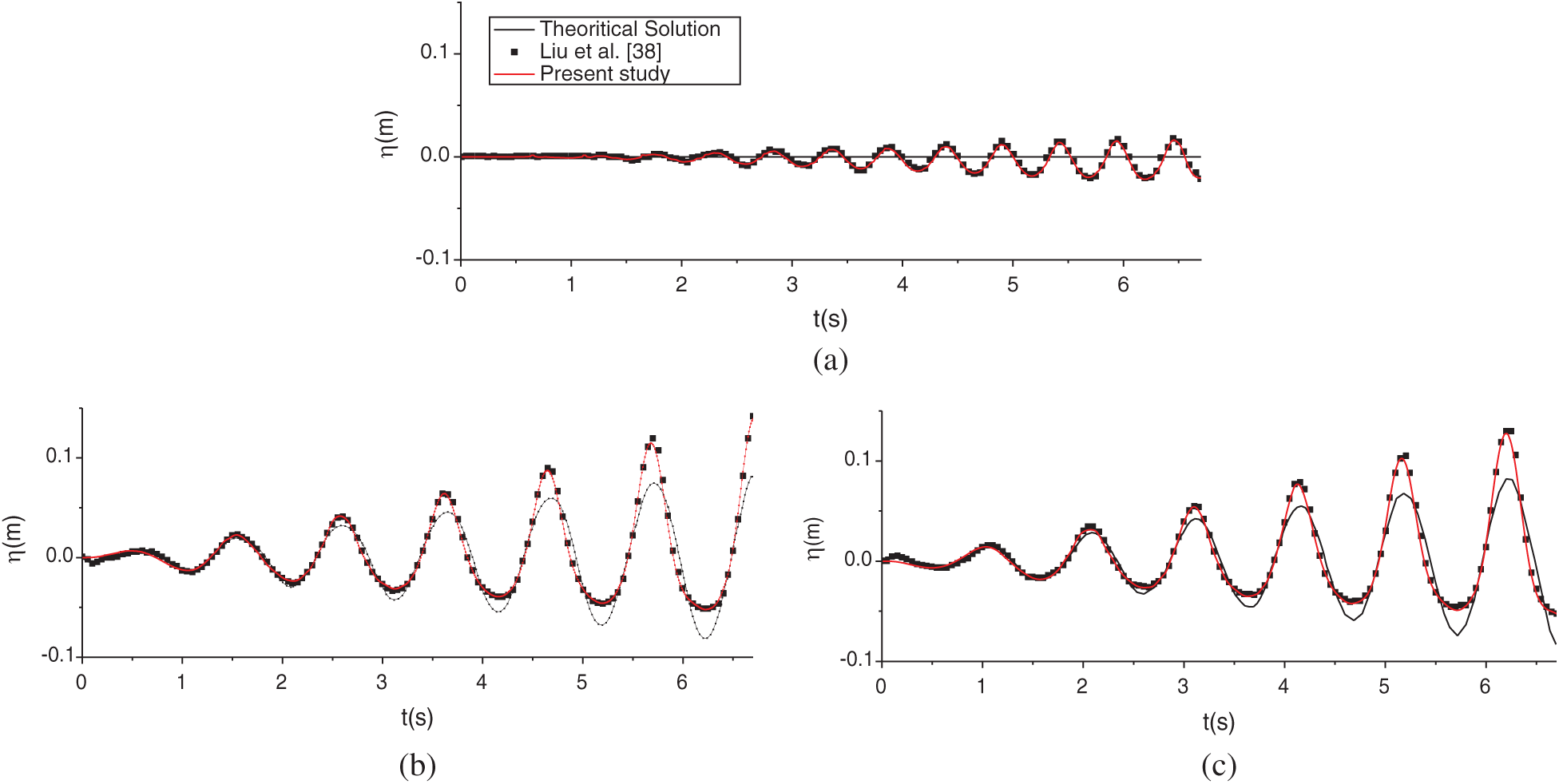
Figure 12: Time histories of free surface height at the gauges: (a) Gauge 1; (b) Gauge 2; (c) Gauge 3

With time going on, the wave amplitude will increase continuously until wave breaking occurs. Two selected moments are given in Fig. 13. Wave overturning and breaking occur on the left and right walls.

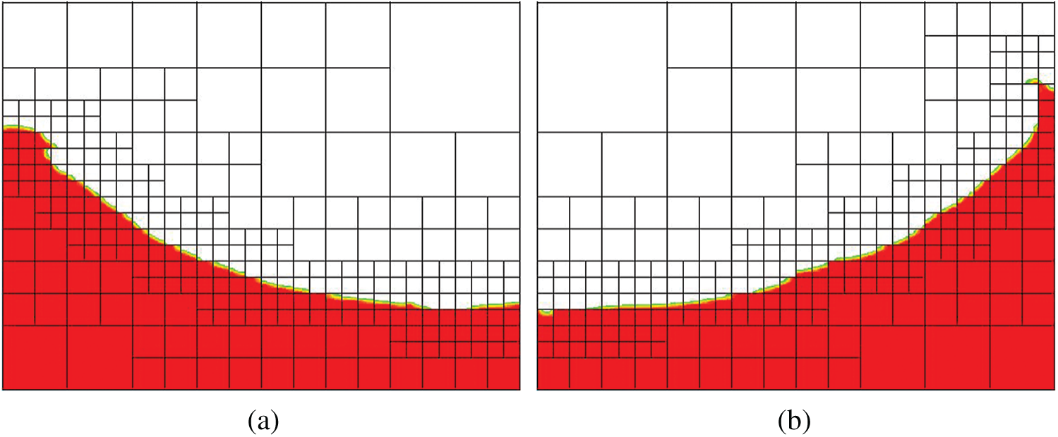
Figure 13: Wave overturning and breaking on the left and right wall: (a) t = 7.8 s; (b) t = 8.2 s

The efficiency of the AMR grid is discussed with this problem. An AMR grid with more levels usually leads to a smaller computational cost, if the minimum scale of the grid is set to be the same. To discuss it in quantitative, the stable phase of the nonlinear sloshing problem is selected (t = 6~8 s). Four grids with different levels (1 to 4) are considered and the finest grid scales are kept the same. The number of grid blocks varying with time is given in Fig. 14. Obviously, a grid with more levels leads to a smaller grid block number.

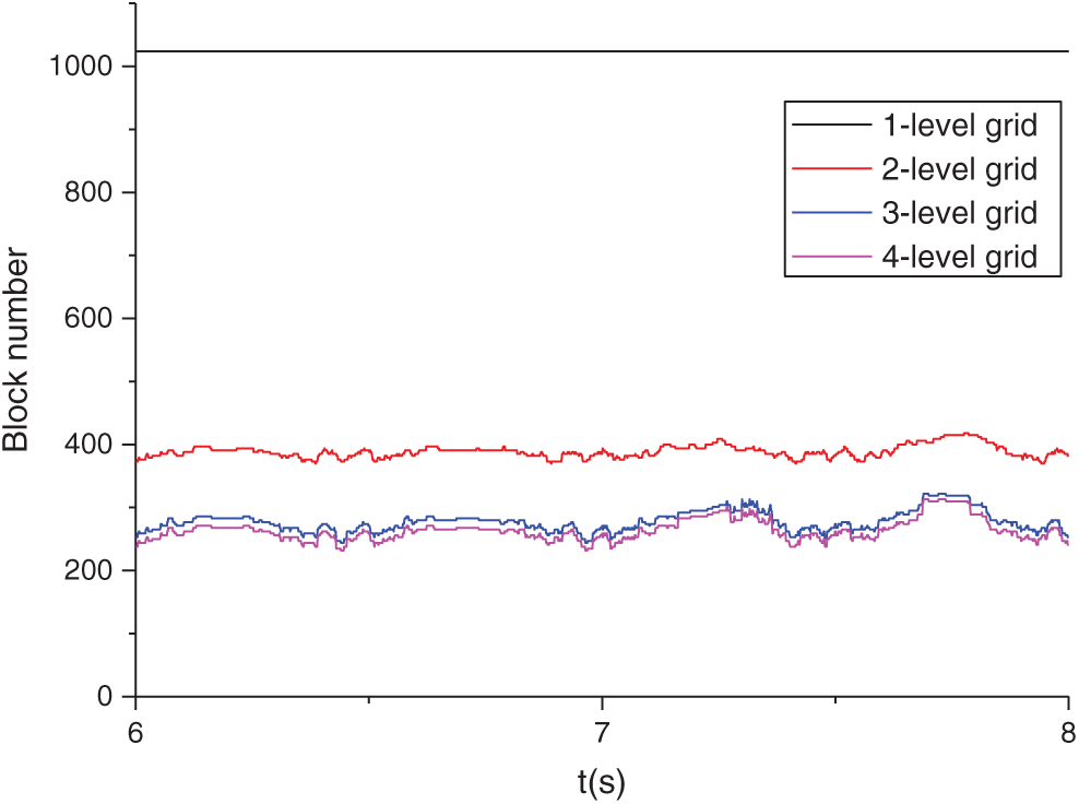
Figure 14: Time history of the grid block number for the four grids

The mean block number and corresponding CPU time for the four grids are shown in Tab. 1. With a 2-level AMR grid, more than 60 percent in grid number and more than 50 percent in CPU time are saved than the 1-level grid (uniform grid). More levels mean more savings and 70 percent in grid number and more than 60 percent in CPU time are saved for the 3-level and 4-level grid. The differences between the save in grid number and save in CPU time is also given in the Tab. 1. The difference increase with the increase of level, due to the increasing coarse-fine interface interpolation and refine/de-refine process for more level grids.

4  Results

In this section, two selected cases are utilized to show that the model is able to simulate violent interface problems.

4.1 2D Solitary Wave Past a Submerged Stationary Stage

To demonstrate the model’s ability in dealing with wave breaking problems, a solitary wave past a submerged stationary stage is considered with the model. The computational model of the problem is shown in Fig. 15 with the parameters to be the same as the experiment conducted by Yasuda et al. [40]. Three gauges are set in the zone, referred to as P2, P3, and P4 by Yasuda et al. [40], respectively. The same problem was also considered by Lubin et al. [41] numerically.

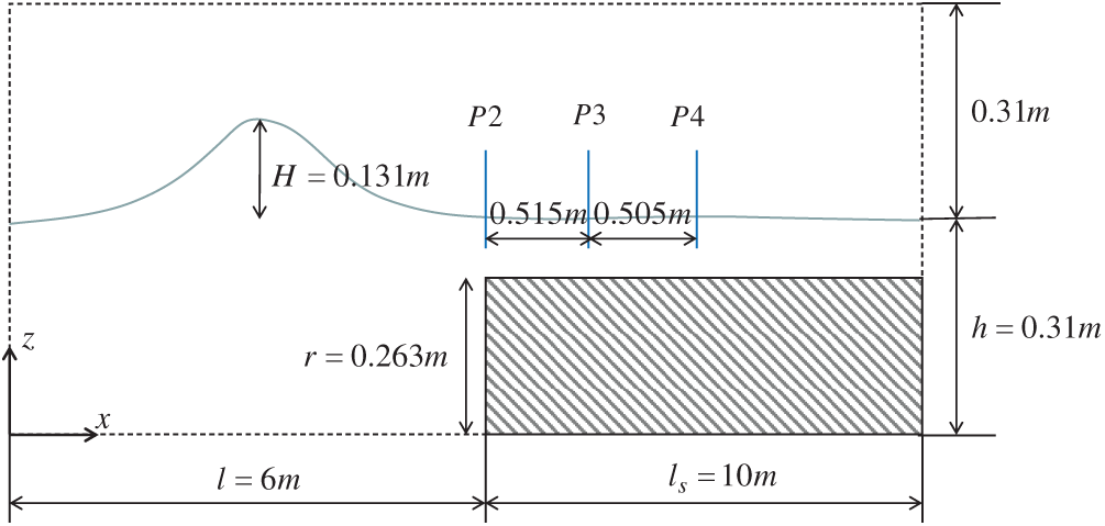
Figure 15: Computational model for solitary wave past a submerged stationary stage

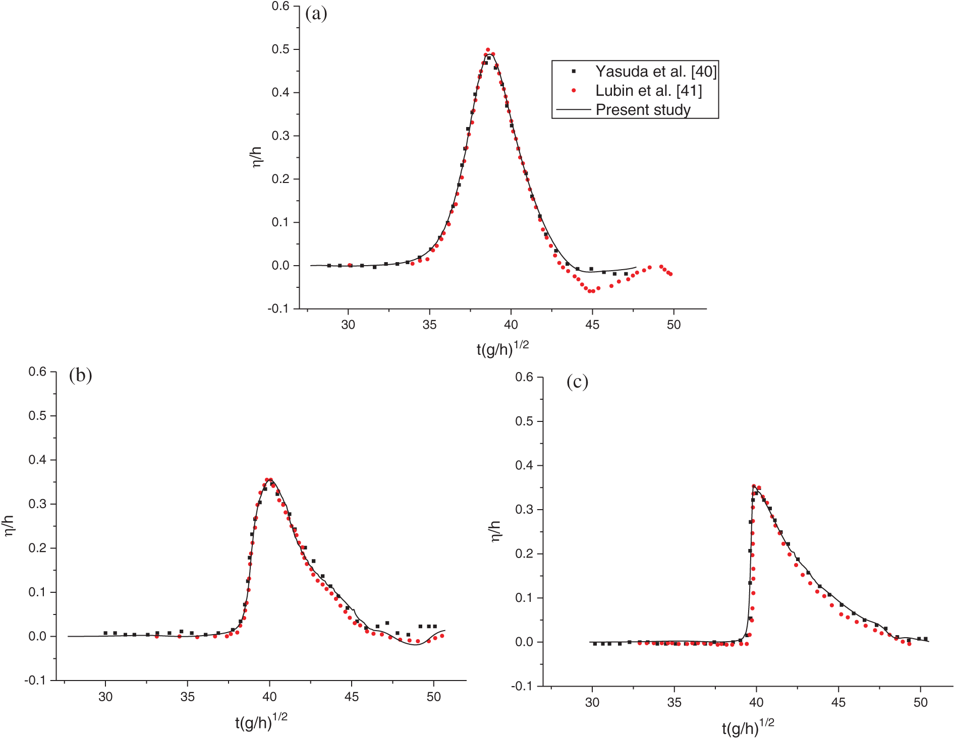
Figure 16: Time histories of free surface height at the gauges: (a) P2; (b) P3; (c) P4

A 4-level AMR grid is employed and a fixed time step of 0.001 s is adopted for the simulations. The minimum grid scales of the medium grid is 4.8×10−3 m on both horizontal and vertical directions after a careful convergence test. The time histories of free surface height at the gauges are compared with the experimental data from Yasuda et al. [40] and the numerical results from Lubin et al. [41], as shown in Fig. 16. All the results achieve good agreement including gauge P4, for which the free surface increases suddenly due to the existence of the stage.

Wave profiles at selected moments are shown in Fig. 17. The wave profile at the forehead becomes up straight first (Fig. 17a). Then the forehead rolls over as shown in Fig. 17b. The process means the current wave breaking mode is plungers [42].

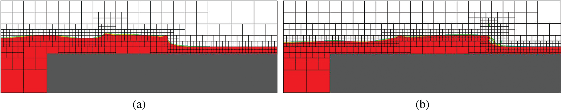
Figure 17: Wave profiles at selected moments: (a) forehead up straight; (b) forehead rolls over

4.2 2D/3D Dam Break

Dam break is a typical violent free-surface flow problem, as complicated phenomena including merging, overturning, and air entrainment occur during the process. The problem was studied by Martin et al. [43] experimentally, and then by researchers in various ways [44,45]. The computational layout of the 2D dam break problem is shown in Fig. 18, with a = 0.2 m corresponds to the parameters of Hu et al.’s [45] experiment. For the 3D case, the spanwise scale is a.

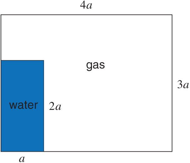
Figure 18: Computational layout of the dam break problem

Both 2D and 3D simulations are conducted, with the minimum grid scale to be 1/128 and 1/64 for 2D and 3D, respectively. A constant time step of 0.001 s is used. The water is initially at rest (t = 0 s) and then moves under the influence of gravity force. Time histories of wavefront location and water column height are presented in Fig. 19. Results on the three grids are compared with the experimental data of Martin et al. [43], Hu et al. [45], and the numerical results of Ubbink [46]. The results are non-dimensionalized with corresponding parameters to ease the comparison. It is observed that the results agree well with the experimental data and numerical results from other sources.

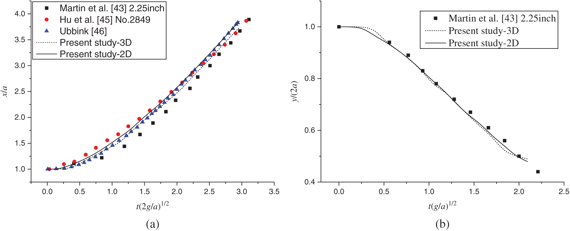
Figure 19: Comparison of non-dimensional time histories of: (a) the wavefront location; (b) the water column height

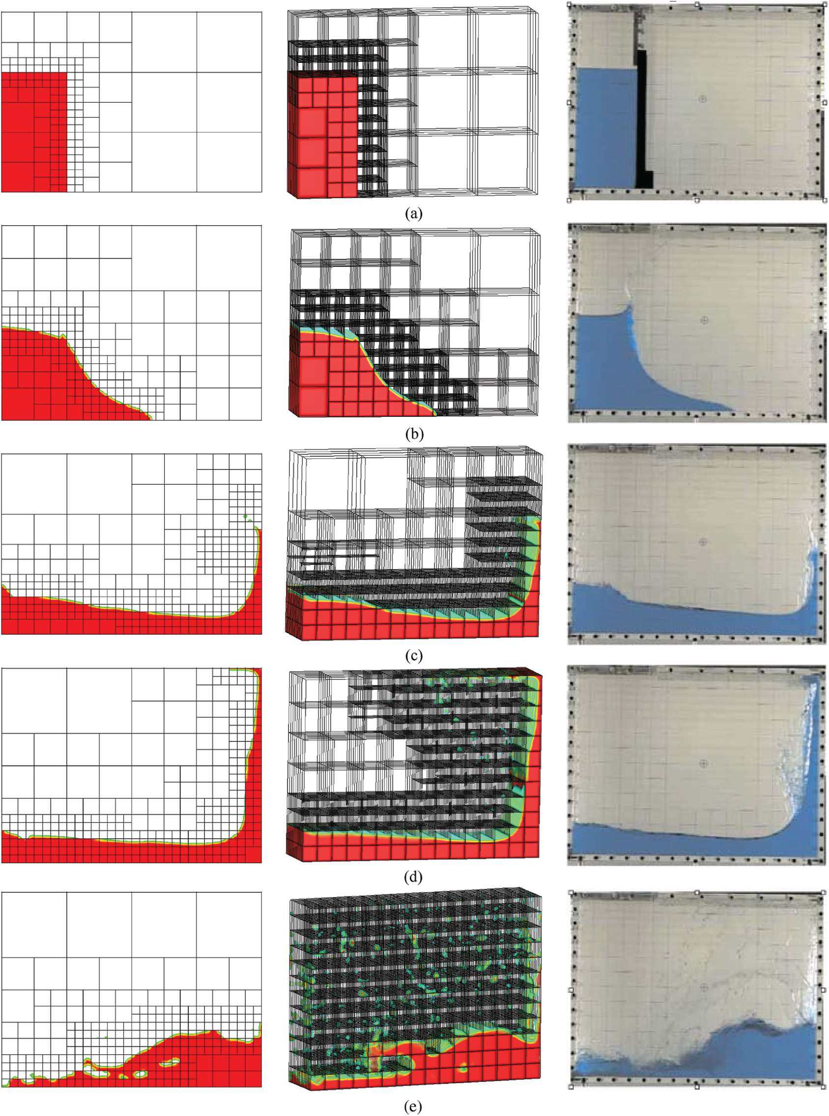
Figure 20: Comparison of the water run-up and overturning process (left: 2D results; medium: 3D results; right: experimental data from Hu et al. [45]). (a) t = 0.0 s, (b) t = 0.18 s, (c) t = 0.39 s, (d) t = 0.52 s, (e) t = 0.99 s

When the wavefront reaches the vertical wall on the right side, the water will run up and overturn. The process is shown in Fig. 20 with selected profiles, which are compared with the experimental data from Hu et al. [45]. The wavefront reaches the right wall and run-up along the wall (Fig. 20c). Then the water hits the roof with a jet formed (Fig. 20d). Finally, the water overturns to the bottom of the tank, with some bubbles exist in the bulk (Fig. 20e). It is observed that the present results agree well with the experimental data from Hu et al. [45].

5  Conclusions

A numerical model for simulating two-phase flow is developed with AMR. An explicit projection method is used to decouple the velocity and pressure. The free surface is captured with the VOF method combined with PLIC. A coarse-fine interface treatment method is developed to preserve the flux conservation at the interfaces. The adaptive grid is managed with the open-source PARAMESH library.

Several benchmark cases are considered to validate the model. The VOF method is validated with the shear flow test. The accuracy of the model is validated with a linear sloshing problem, for which analytic solutions can be derived. The model is demonstrated to have 2nd-order accuracy in space. The efficiency of AMR is demonstrated with a nonlinear sloshing problem.

The ability of the model to simulate more complex problems is demonstrated with two selected cases including solitary wave breaking and dam break. Good agreements are obtained between the current numerical results and experimental or numerical results from other sources. It is demonstrated that the model is able to simulate interface problems with wave breaking.

Acknowledgement: The authors are grateful for the important and valuable comments of anonymous reviewers.

Funding Statement: This work was financially supported by the National Natural Science Foundation of China (Nos. 51779049, 51879058, 52071098, 51979053).

Conflicts of Interest: The authors declare that they have no conflicts of interest to report regarding the present study.

This work is licensed under a Creative Commons Attribution 4.0 International License, which permits unrestricted use, distribution, and reproduction in any medium, provided the original work is properly cited.