Computer Modeling in Engineering & Sciences

DOI: 10.32604/cmes.2021.015159

ARTICLE

The Research of Automatic Classification of Ultrasound Thyroid Nodules

Yanling An1, Shaohai Hu1,*, Shuaiqi Liu2,3, Jie Zhao2,3,* and Yu-Dong Zhang4

1Institute of Information Science, Beijing Jiaotong University, Beijing, 100044, China
2College of Electronic and Information Engineering, Hebei University, Baoding, 071000, China
3Machine Vision Technology Innovation Center of Hebei Province, Baoding, 071000, China
4Department of Informatics, University of Leicester, Leicester, LE1 7RH, UK
*Corresponding Authors: Shaohai Hu. Email: shhu@bjtu.eud.cn; Jie Zhao. Email: zhaojie_hbu@163.com
Received: 26 November 2020; Accepted: 01 March 2021

1  Introduction

Thyroid nodule is a common disease and timely detection and treatment can prevent it from turning into malignant tumors. The continuously improved accuracy of ultrasound diagnosis of thyroid nodules has made ultrasound diagnosis the preferred laboratory examination of thyroid nodular disease [1,2]. In the process of detecting and assessing disease severity, computer-aided analysis [3,4] improves the readability of medical images and provides a reliable second opinion, which helps doctors to make a more accurate diagnostic decision. Computer-aided diagnosis system has been successfully applied to the analysis of ultrasound images of liver, breast, prostate and other soft tissues of different internal organs. Currently, comparatively fewer researches apply computer-aided analysis to assess thyroid diseases. And early studies on thyroid texture analysis are limited to extracting features from histograms. For example, Iakovidis et al. [5] proposed a fuzzy local binary pattern (FLBP) for ultrasound texture characterization to automatic classification of thyroid nodules. Chang et al. [6] applied support vector machine for feature selection and classification of thyroid nodules in ultrasound images. Morifuji et al. [7] studied whether thyroid nodules are malignant; Acharya et al. [8] combined local binary pattern (LBP) and Gabor transform features for automatic classification of ultrasound thyroid nodules. On one hand, these studies demonstrated the effectiveness of histogram on thyroid tissue feature. On the other hand, the feature-based histogram cannot compile the distribution of the image pixels on space. Thus, for thyroid ultrasound image texture analysis, the new approach combines histogram features with statistical features. These statistical features include Haralick co-occurrence features [9,10], Muzzolini spatial characteristics [11], Radon transform features [12] and LBP features [13]. Most of these methods use histogram, second or even senior statistical texture descriptors to indicate thyroid ultrasound mode. In order to consider the uncertainty caused by the inherent speckle noise of thyroid ultrasound images, Iakovidis et al. [14,15] proposed FLBP algorithm. But the selection of fuzzy parameters increases the feature dimension, which, is not conducive to the classification hyperplane search from the classification point of view. Moreover, the training costs will be greatly improved, while the speed of classification will be appropriately reduced.

To sum up, the diagnosis of thyroid disease is mainly carried out through studying the ultrasonic image texture features and the echo pattern at home and abroad. Research based on shape information is rare. Therefore, this paper makes quantitative analysis and study on morphological characteristics. Description of thyroid nodules’ morphological characteristic parameters is extracted and fused with texture and gray feature to analyze thyroid, so as to discriminate the tumor as benign or malignant. It offers a reference for the clinical thyroid nodule detection and diagnosis.

2  Segmentation of the Nodules’ Region

With the advantages of automatically processing topology changes, active contour segmentation based on level set becomes a widely used method in the field of image segmentation [16,17]. The basic idea is to represent contour as the zero-level set of the level set function, then the level set function is embedded to the curve evolution equation. The evolution of the curve is obtained through the evolution of its zero-level set. In this paper, we choose the classic DRLSE model as the prototype of the segmentation model. The relevant theoretical of the DRLSE model and the disadvantages existing in practical application will be described as follows.

2.1 DRLSE Model and Analysis

The DRLSE model, proposed by [18], is a variational level set partitioning method based on edge information. Its energy functional is as follows:

ε(ϕ)=μRp(ϕ)+λL(ϕ)=μ∫Ωp(∇ϕ)dx+λ∫Ωgδ(ϕ)∇ϕdx (1)

where ϕ is the level set function, ε is the energy functional form, Rp is the distance adjustment term of the level set, ∇ is Laplacian operator, Ω is the local region of image, and p is energy density function. At last, μ and λ are respectively the weight coefficients of the regularization term and the length term. The first item is the regularization term of the level set function ϕ regularization term is to ensure that the level set function ϕ is approximately to the signed distance function to the greatest extent during the curve evolution, which avoids periodic initialization of curve evolution in the evolution process. The second term is weighted length term which takes the g function as the weight. It is used to drive zero-level set curves to evaluate to the target edge. Based on the image gradient, theg function is an edge-stopping function which can be obtained by:

g≜11+|∇Gσ∗I|2 (2)

where Gσ is the Gauss filter function, I is the image, and ∇ is the gradient operator.

DRLSE model features simple numerical solution and speedy convergence. Moreover, it does not need to reinitialize the level set. However, for the segmentation of medical ultrasound images, due to the low contrast between tissues and organs in ultrasound images, fuzzy boundary, intensity inhomogeneity in images before and after ultrasonic field, the g function cannot reach zero on the boundary, while curve evolution can not stop at the target boundary. As shown in Fig. 1, a thyroid nodule ultrasound image. We put the initial contour inside the target and evolve it through expansion curve. The experimental results show that the curve evolution crosses the target boundary, leading to edge leakage.

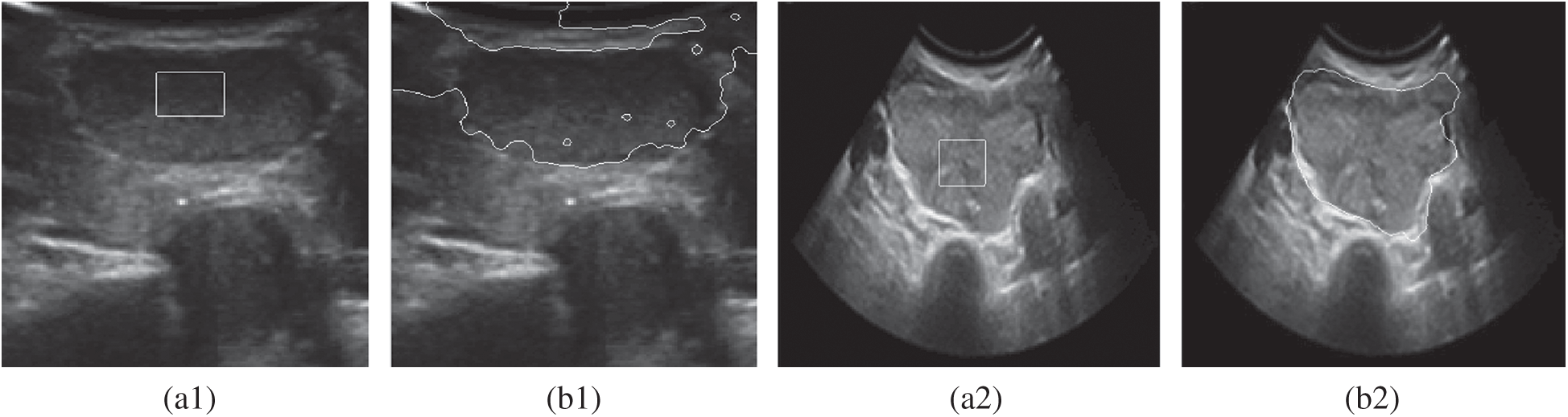
Figure 1: A comparison of the inaccurate boundary locations of the DRLSE model. (a1) Original image1 (b1) DRLSE segmentation (a2) Original image2 (b2) DRLSE segmentation

The problem is that when an edge-stopping function deals with weak edges, it is not zero at the weak edge due to the relevant small gradient of the weak edge [19]. Therefore, it is necessary to search for a new edge-stopping function which can guarantee the convergence at the weak boundary.

Considering the importance and the stability of the phase information, this paper tries to use phase information to segment the thyroid ultrasound image. We design an edge-stopping function that combines phase information with gradient information, replace the edge-stopping function based on gradient in DRLSE model and solve the problem that the evolution curve cannot be stopped at the target boundary in DRLSE model.

2.2 Phase Coherence Thyroid Nodule Segmentation Analysis

The phase congruency detection is a new method to detect features. Rather than detecting based on intensity gradient features, it analyzes the mutation location of image gray level from the frequency domain [20]. Studies have shown that image features perceived by human eyes are often located in the high point of phase congruency, while edge detection of phase congruency is assumed that the most congruent phase points of the Fourier components in the image were feature points. Thus, edge detection is a more reliable way than the conventional gradient calculation method. Based on this principle, Morrone et al. [21] defined the phase congruency function:

PC(x)=maxφ(x)∈(0,2π)∑nAncos⁡(φn(x)−φ(x))∑nAn (3)

where PC(x) is the phase congruency measure, obtaining maximum value at the target edge while obtaining a smaller value in the background area with its value which ranges from 0 to 1, An represents the magnitude of the n-th harmonic cosine component. φn is the initial phase of the second component of n, φn(x) represents the local phase point of the Fourier components of the point x. Fig. 2 is the experimental results comparison between the gradient detection and phase detection of the thyroid ultrasound images. We can find the phase congruency performs better than gradient operator in detecting the edge of the target.

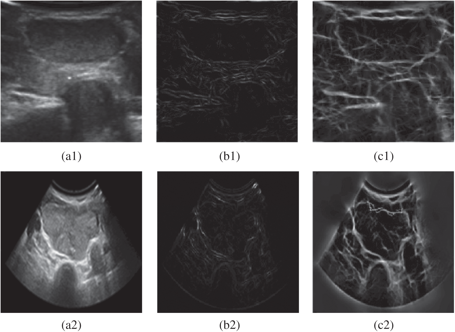
Figure 2: Experimental comparison chart of gradient edge detection and phase detection. (a1) Original image (b1) Gradient edge detection (c1) Phase edge detection (a2) Original image (b2) Gradient edge detection (c2) Phase edge detection

Therefore, a boundary indicator function based on the phase congruency operator and gradient operator is proposed in this paper. Let I be the image and I(i,j) is the gray level of the pixels in i-th row and j-th column in image I, and the phase PC(i,j) is the phase congruency function value of the i-th row and j-th column. At the edge of the image, phase congruency of the image is relatively larger, which is pc(i,j)≥k. k is the manually set constant, which is set to 0 on this occasion. Phase congruency is smaller in the flat areas of the image. To avoid trapping into local minimum value, we still choose edge-stopping function based on gradient. Therefore, combining phase information with gradient information, we construct a new edge indicating function gp(I) (also called edge-stopping function) acting as edge stopping power, which forces the level set evolution curve stopping at the target edge. The function is specifically defined as follows:

gp(I)={11+|∇I(x,y)|2,pc(i,j)≤k0,pc(i,j)≤k} (4)

In light with the Fig. 3, a 3D comparison of the effects is shown. The comparison is between the original edge-stopping function based on the gradient information and the edge-stopping function combining the phase information with the gradient information for thyroid ultrasound images at the tumor edge. It can be seen that the improved boundary function convergent at the weak boundary.

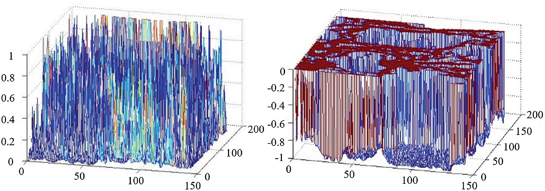
Figure 3: 3D effect comparison between gradient edge detection and phase detection

2.3 Level Set of the Segmentation Model Improvement

Based on geometric evolutionary theory and partial differential equations theory, we use boundary indicator function gp(I) that combines the phase information with gradient information to control the curve evolution. We construct a new energy functional as follows:

ε(ϕ)=μRp(ϕ)+λL(ϕ)+αA(ϕ)=μ∫Ωp(∇ϕ)dx+λ∫Ωgδ(ϕ)∇ϕdx+α∫ΩgH(−ϕ)dx (5)

where ϕ is the level set function, ε is the energy functional form, Rp is the distance adjustment term of the level set, ∇ is Laplacian operator, Ω is the local region of image, and p is energy density function. At last, μ, λ and α are respectively the weight coefficients of the regularization term, the length term and the area term. H is the Heaviside function and δ is the Dirac function. The first item is the regularization term of the level set function ϕ regularization term is to ensure that the level set function ϕ is approximately to the signed distance function to the greatest extent during the curve evolution, which avoids periodic initialization of curve evolution in the evolution process. The second term is weighted length term which takes the g function as the weight. It is used to drive zero-level set curves to evaluate to the target edge. The third term is the weighted area term which takes the g function as the weigh. It corresponds to the balloon force and is used to speed up the evolution. When the initial contour is outside of the target, α takes a positive value which could make the contour rapidly shrinks. While the initial contour is inside of the target, α takes a negative value which could make the contour rapidly expanses. Based on the image gradient, the g function is an edge-stopping function According to the variational theory, the gradient descent flow of the steepest descent of minimize functional ε is:

∂ε∂ϕ=μ[Δϕ−div(Δϕ|Δϕ|)]+λδ(ϕ)div(gpΔϕ|Δϕ|)+αgpδ(ϕ) (6)

The descent flow equation is the evolution equation of the level set segmentation model that combines the phase with gradient information. Fig. 4 shows the effect of image segmentation of the above algorithm.

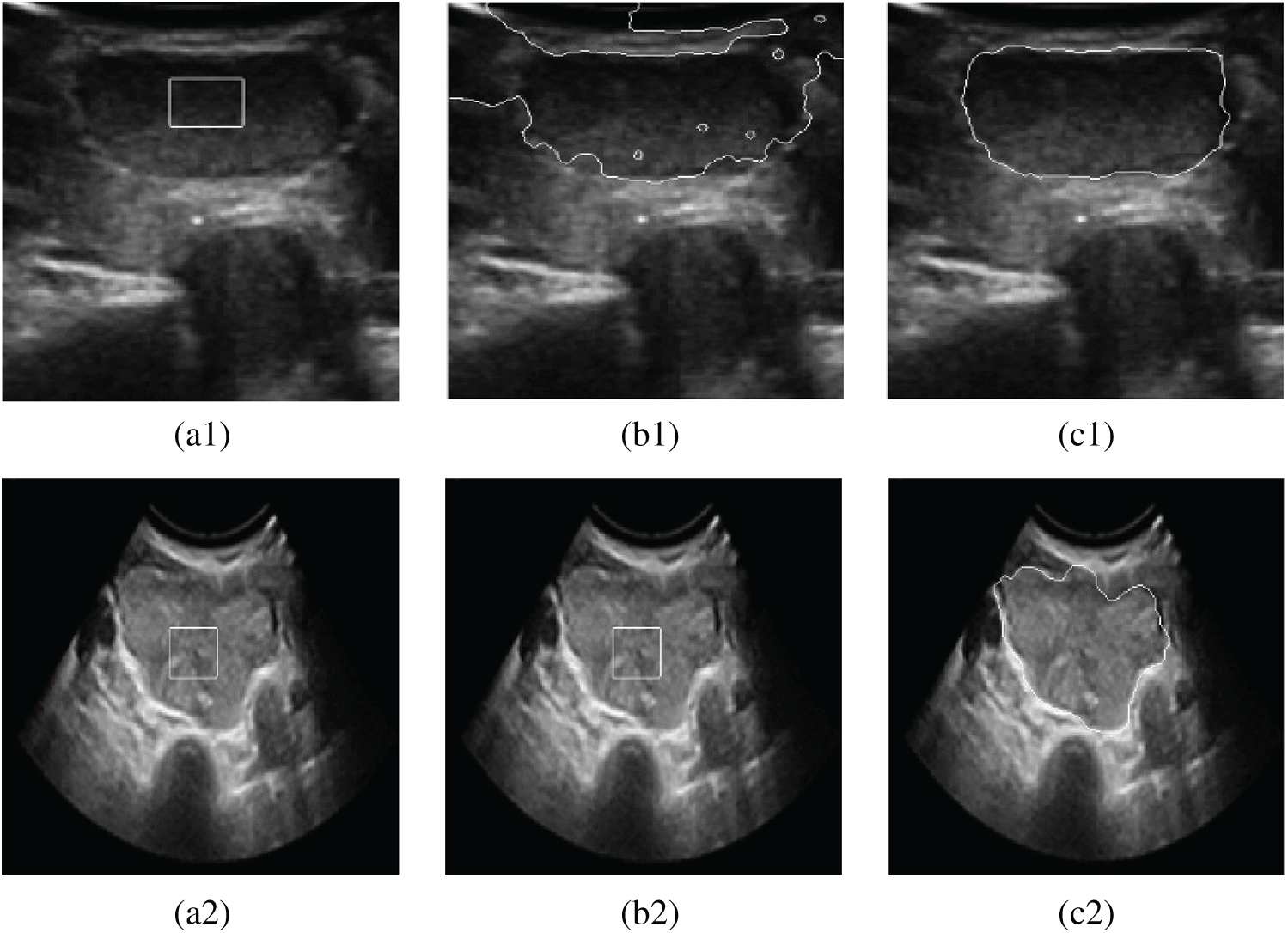
Figure 4: Contrast segmentation results of thyroid ultrasound images. (a1) Original image 1 (b1) DRLSE model (c1) The proposed model (a2) Original image 2 (b2) DRLSE model (c2) The proposed model

3  Feature Extraction

On the basis of segmentation, the feature extraction of nodules is carried out. In clinic, doctors discriminate the thyroid nodules as malignant or benign according to nine parameters: morphology of nodules, boundary, capsule, acoustic halo, depth-width ratio, internal echo, calcification spot, rear echo and blood flow. Among these features, shape, boundary, capsule, acoustic halo and depth-width ratio can be described through contour feature extraction of the nodules. While internal echo, calcification spot, rear echo can be described through the gray and texture since they are related to the gray distribute on of thyroid nodule ultrasound image. Therefore, this paper puts forward a new feature extraction algorithm that combines the feature of the information of shape, texture and gray of the ultrasonic image for discrimination of benign and malignant thyroid nodules.

3.1 Shape Feature Extraction

On the basis of segmentation, contour features of nodule, including shape, orientation and edge, extract the features of nodules’ circularity, depth-width ratio, the average direction number, the standard deviation of the normalized radial length, roughness index and envelope and acoustic halo [22]. The circularity, the average direction number and the standard deviation of normalized radial length of nodules are parameters which are associated with the nodule shape (reflecting the irregular degree of nodules). The depth-width ratio reflects the growth pattern of nodules. Roughness index describes the nodules (Burr) edge, while envelope and acoustic halo features reflect whether the nodules have envelope and acoustic halo or not.

(1) Circularity (Roundness)

Assuming that the whole area of the tumor is S and the perimeter is L, we define the circularity as:

E=4πS/L2 (7)

Image is composed of pixels, so L can be represented by the number of pixels on the edge. S can be represented by the number of pixels on the edge. The closer to circle the tumor shape is, the bigger E value will be, and the more likely the tumor is benign, and vice versa.

(2) Standard deviation of the normalized radial length

The distance between the centroid of the tumor area and the edge of the image is considered as the radial length of the tumor, as shown in Fig. 5.

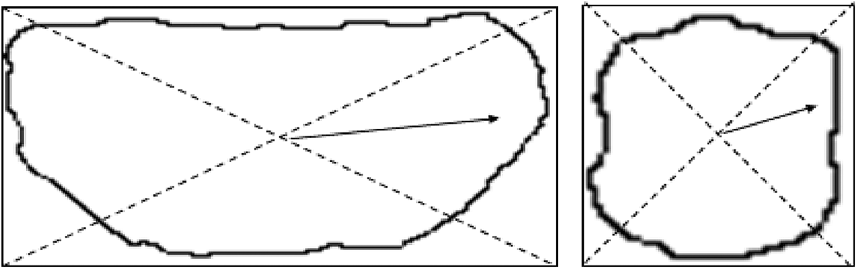
Figure 5: Radial length schematic diagram

Normalized radial length is obtained by normalizing the radial length, as shown in the following:

d(i)=(x(i)−x0)2+(y(i)−y0)2max(d(i)),i=1,2,⋯,N (8)

where (x0,y0) is the centric coordinates, (xi,yi) is the coordinates of i-th point on the edge of tumor. N is the number of points on the tumor edge. max(d(i)) is the maximum value in radius. Therefore, the average value dave and the standard deviation std of the normalized radial length are obtained by the following calculation:

dave=1N∑i=1Nd(i) (9)

std=1N−1∑i=1N(d(i)−dave)2 (10)

The principle that discriminates benign and malignant tumor through the standard deviation of normalized radial length macroscopically reflects the similarity between the contour and the circle.

The smaller the standard deviation is, the more similar to circle the target is, and the more likely is benign tumor.

(3) Average direction number

In the process of edge extraction, we set the angle between any pixel and the adjacent pixel as αi, the number of pixels on the image edge as N. The average direction number is defined as:

D=∑i=1Nαi/N (11)

The average direction number is mainly used to reflect the smooth degree of the tumor edge, the smoother the edge is, the smaller the average direction is.

(4) Depth-Width Ratio (DWR)

In clinical, DWR is a frequently applied quantitative feature of thyroid ultrasound. Depth represents the distance between the furthest two points on the edge. Width represents the distance between the nearest two points on the edge. DWR is defined as:

DWR=DepthWidth (12)

In some extent, it reflects the growth pattern of tumor. It is generally considered that if the DWR is less than 1, the malignant degree of tumor is low.

(5) Boundary roughness R

R=1N∑i=1N|d(i)−d(i+1)| (13)

The roughness is the average of the sum of the absolute value of the difference of standard radius of the adjacent two points on the edge in clockwise or counterclockwise direction. Obviously, the rougher the edges are (and sometimes more Burr), the bigger value it will be, and the more likely for it is cancer.

(6) The envelope and acoustic halo feature

The description of the edge feature of benign nodules generally involves envelope and acoustic halo. The quantification of edge features can be calculated through the gray distribution [23] at the adjacent areas of the nodules’ boundary. In the level set method, two strip areas which locate inside and outside of the nodule can be obtained. We respectively took a level set function −0.5, 0 and 0.5, among which the level set −0.5 corresponds to the nodule interior, level set 0 corresponds to the nodule boundary and level set 0.5 corresponds to the nodule exterior, as shown in Fig. 6.

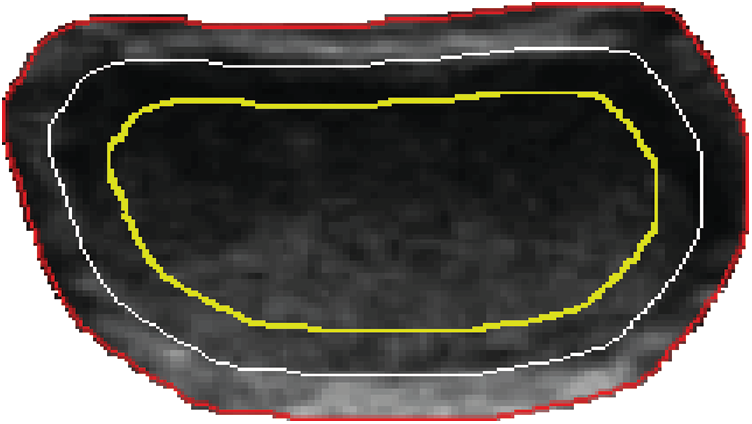
Figure 6: Strip areas in and out of the tumor boundary

Assume that the numbers of pixel in the internal and external strip areas are n1 and n2, and the gray mean values are u1 and u2. We use inter variance to measure the gray statistical differences between the internal and external areas:

InterVar=n1(u1−u)2+n2(u2−u)2(n1+n2) (14)

where u=n1u1+n2u2n1+n2. The bigger InterVar is, the greater possibility for the gray level of internal, the more statistically significant difference external adjacent areas have, and the more possibility for the envelope and halo exist. By normalizing the processing, InterVar is independent with the gray level and the average separability is defined as:

AveSep=InterVarTotalVal (15)

where TotalVar is the variance of the gray level of all pixels of the internal and external strip areas. The maximum of the average separability AvgSep is 1.

3.2 Gray Feature Extraction

Two frequently used clinical features are extracted based on the gray information of the ultrasound image of thyroid gland, which are attenuation coefficient (AC) and micro calcium degree.

(1) Attenuation coefficient

Posterior echo is an important criterion for clinicians to diagnose thyroid tumor. For benign tumors, posterior echo is obviously enhanced. And for malignant tumors, posterior echo is obviously attenuated. Hence, we use the attenuation coefficient to do quantitative processing. A rectangular region of interest is selected from the direction which the tumor region and its posterior echo region appear the biggest change. The attenuation coefficient is defined as the average gray level ratio of the tumor region and the posterior echo region. The average gray levels of region of interest (ROI) in tumor area and posterior echo area are:

MITumor=∑y=0H−1∑x=0W−1ITumor(x,y) (16)

MIEcho=∑y=0H−1∑x=0W−1IEcho(x,y) (17)

where the height and width of ROI are H and W, respectively, x and y are expressed as the pixel coordinates, ITumor(x,y) represents the gray level of the pixels in ROI of the tumor area and IEcho(x,y) is the gray level of the pixels in ROI of the posterior echo area. So the attenuation coefficient named AC is defined as:

AC=MITumorMIEcho (18)

(2) Micro calcification degree

Calcification in the nodule is a common feature in thyroid ultrasound images. Calcification can be divided into three types: Micro calcification: ≤1100 um pinpoint-ish strong light spots; Coarse calcification: >1100 um strong light cluster; Arc calcification: the surface of the bump which is curved or the ring of the bright band accompanied by sound shadow. Calcification plays an important role in differentiating thyroid cancer, and different calcification patterns have different clinical significance. This paper uses the pixel gray level to measure the intensity of light spots and the number of pixels to calculate calcification area and measure whether the calcification is micro calcification or not. Moreover, this paper proposes a micro calcification degree measuring method which is specific to thyroid nodule. As gray information of ultrasonic image is easily influenced by instrument, the average of total pixel gray level within nodules is taken as a reference in this paper. By calculating the average pixel gray level within nodules and the pixel gray level within calcified plaque, we work out the relationship between them to draw a conclusion. We define the strong light spot whose pixel gray level within nodules is larger than 200% as the calcification point. Binarization processing is carried out for the strong light spots and the non-strong light spots, forming m regions of strong light cluster with the pixel number in each region being denoted by ni, i=1,2,⋅⋅⋅,m. Then we calculate the area of light spots in the cluster region and niS. If the result is smaller than a threshold value γ, then the cluster area is micro calcific, where γ=1.21×106 um2 means the area of micro calcification based on medical judgment and w micro calcification regions will be got. The micro calcification degree is defined as the ratio of the area of micro calcification region within the nodules and the number of pixels in the region of calcification within the nodules:

Cal=∑j=1wnj∑i=1mni (19)

The micro calcification degree can well reflect the existence and degree of micro calcification in the nodules. Cal∈[0,1], if micro calcification degree is 0, then no micro calcified plaque exists in the nodule. There is no statistical significance using calcification feature to diagnose benign and malignant nodules. The higher degree of micro calcification is, the greater possibility of malignant nodules has.

3.3 Texture Feature Extraction

3.3.1 Local Two Valued Pattern

Deriving from a definition of local neighbor texture, the local binary pattern is a texture measurement within the gray scale [24]. It uses the structural method to analyze the fixed window features and the statistical method to extract the whole feature. The initial LBP operator is defined as: set one pixel f(xc,yc) in a local region in the image as the center point gc, which combines with the eight pixels points g0,⋯g7 within its surrounding 3×3 window, forming a texture primitive T={gc,g0,⋯,g7}. Taking the gray level of window center point gc as the threshold, the gray level of the adjacent eight pixels is compared with the threshold, if the gray level of the adjacent pixels is greater than that of the threshold, then the pixel position is 1, otherwise, it will be 0. Thereby a series of binary values di(0≤i≤7) are achieved, as shown below:

di={1ifΔgi≥00ifΔgi<0 (20)

where Δgi=gi−gc. After this process, the 8-pixel points within the 3×3 window can generate a binary code of 8 bits, and then a binary number of 8 bits can be read in a clockwise direction. Through giving different weights to different positions, the 8-bit binary code can be switched to an unsigned integer, namely switching it to decimal number according to the formula (20). This number is defined as the LBP value of the window, reflecting the texture information of the region, that is, the LBP code value which describes the spatial structure characteristic of local image texture is expressed as:

LBP=∑i=07di∗2i (21)

Theory of LBP algorithm is simple, while it can reflect the subtle variations among texture without parameter setting problem getting involved. Comparing with other methods, it is a fast and efficient texture description operator. However, it is obviously unreasonable if all cases are treated with single mapping transformation. For example, if the center pixel gray level is 60, while its adjacent pixel’s gray level is 59. In this case, coding the pixel as 0 is obviously unreasonable. Moreover, LBP operator usually applies the LBP histogram as the texture feature of regional description. If feature dimension is too large, from the classification point of view, it causes difficulty in searching the classification hyperplane and improves the training cost. To overcome these shortcomings, literature [14,15] proposed the FLBP algorithm, carrying out fuzzy coding for the distance. But the coding number will increase along with different fuzzy degree, causing the curse of dimensionality. Hence, based on this algorithm, this paper makes an improvement on it. According to sensory awareness, most of the nodules in thyroid ultrasound image are in elliptical shape. We improve the neighborhood and use elliptical local binary pattern (ELBP) to encode the thyroid ultrasound image.

3.3.2 Thyroid Ultrasound Feature Extraction Algorithm Based on Fuzzy Elliptical Local Binary Pattern

(1) The neighborhood improvement

In the ELBP method, the distribution of the neighborhood pixels is in elliptical shape, as shown in Fig. 7. There are three related parameters: ① the axis of the ellipse is denoted by A; ② the minor axis of the ellipse is denoted by B; ③ the number of adjacent pixels is denoted by m.

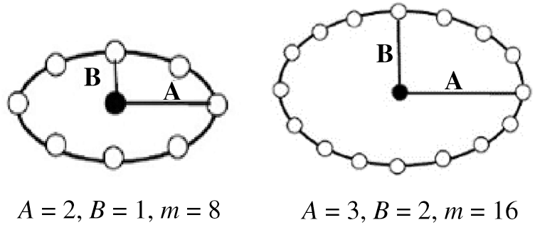
Figure 7: ELBP model example of different parameters

The X, Y coordinates of each neighborhood pixels pi are pix and piy, and their corresponding center pixels are determined by the following formulas:

Ri=A2B2A2sin2⁡θi+Bcos2⁡θi (22)

pix=Ri∗cos⁡θi,piy=Ri∗sin⁡θi (23)

where θi=(360m∗(i−1))∘. The nearest neighbor interpolation method is used on non-integer coordinates to obtain integer coordinates.

(2) The distance coding improvements

We can see in literature [14,15] that the parameter F is introduced to better describe the spatial structure of the local image texture. As described before, classic LBP uses a single LBP code to describe a 3×3 texture primitives, while in FLBP method, a primitive can be described by multiple codes with each LBP code having a corresponding weight WLBP. Bigger weights prove the greater possibility to be LBP patterns, the CLBP of each LBP code is defined as:

CLBP=∏i=07udi(i) (24)

where di∈{0,1}, udi denotes the binary descriptor operation. LBP code values can be obtained by the formula (21), and the total weight relationship of all modes is as follows:

∑LBP=0255WLBP=1 (25)

Based on the above literature, to select the center value more reasonably, we multiply the LBP codes appeared in each texture primitive by its corresponding weight and then sum them and round up the result. The FLBP code value which described the spatial structure of local image texture is obtained expressed as:

FLBP=∑LBP=0255LBP∗WLBP (26)

The improved fuzzy elliptical local binary pattern (FELBP) operator is applied on image processing, and the processed images are shown in Fig. 8.

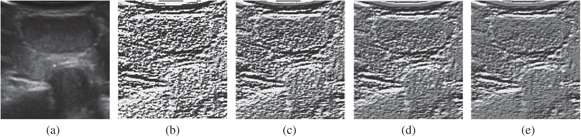
Figure 8: The example results of FELBP operator processing. (a) The original figure (b) F = 0 (c) F = 5 (d) F = 10 (e) F = 15

Fig. 8a is the original image, while Figs. 8b–8e are the FELBP images when the F value is taken as 0, 5, 10, 15, respectively. It can be seen that Fig. 8b, the one with smaller F value, depicts more texture details relatively. At the meantime, its noise is more obvious. Fig. 8e with a larger F value mainly describes the edge outline information of the thyroid image, especially the edge of nodules and the trachea. And some smaller textures are filtered out. Figs. 8c and 8d with middle F values describe the texture information of middle layers. In general, with the increasing F values, detailed texture information in image described by FELBP is gradually weakened, while contour information such as edge information is gradually enhanced.

In order to find the most suitable feature subspace to classify benign and malignant thyroid, we adjust the fuzzy degree parameter F value to seek the best classification performance. Taking F=0,1,2,⋯,15, the statistical FELBP model value of the thyroid ultrasound image is input to SVM [25] classifier of different kernel functions for validation. Fig. 9 is the classification accuracy of different kernel functions with variable degree of fuzzy parameters F. The performance described by F=0 is corresponding with the traditional LBP. Its classification accuracy reaches the highest point of 72.3% under the polynomial kernel function of SVM. For each SVM kernel function, its classification accuracy obtained through FELBP is higher than that through LBP. In the SVM [26] polynomial kernel function, the maximum classification accuracy of FELBP reaches 90.1% when F=10. Thus, we find the optimal feature subspace which is suitable for the classification of benign and malignant thyroid nodule. These improvements solve the problems as single transformation mapping of LBP algorithm and its being sensitive to noise. The problem that the feature dimension being too big is yet to be solved properly. Therefore, this paper extracts the entropy of nodule region as the texture feature. After processing the FELBP algorithm, the nodal region entropy in the processed image is extracted using PFELBP to represent the probability of occurrence of model value FELBP. The entropy represents the texture feature of nodule region and also reflects uniformity degree of the internal echo to a certain extent. The stronger FELBP model value diversification is, the bigger entropy value is, the simpler texture is, and the more uniform internal echo is. If all the parameters of probability are equal, the entropy will achieve maximum. Its entropy is defined as:

ϕ=−∑LBP=0255PFELBPlog⁡(PFELBP) (27)

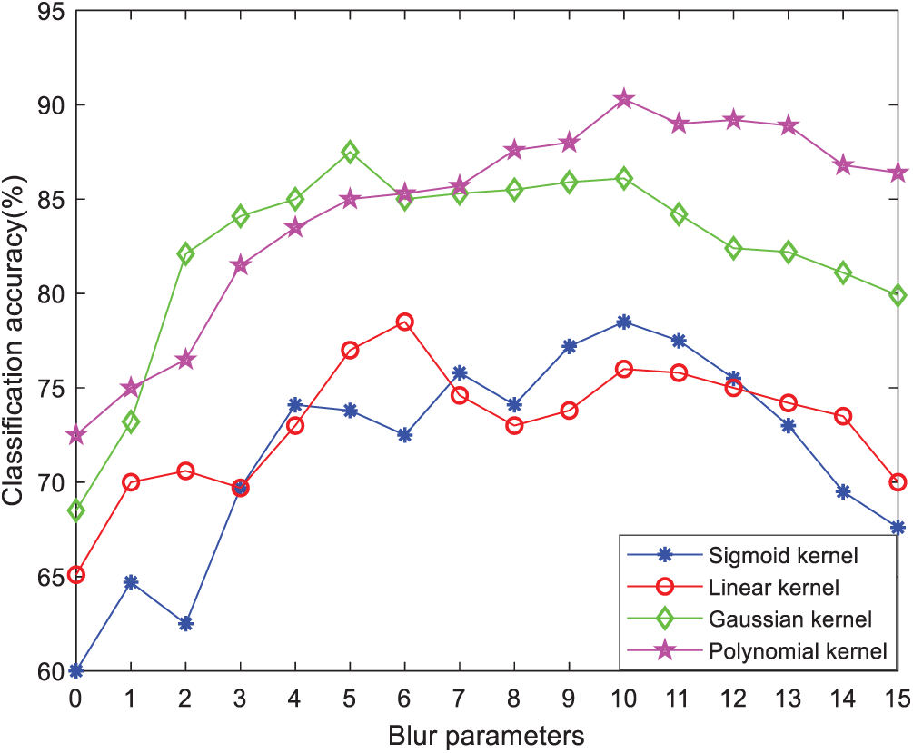
Figure 9: Classification accuracy of different kernel functions with variable degree of fuzzy parameters F

4  The Improved SVM

SVM has good generalization performance in dealing with situations like small sample, nonlinearity and high dimension, which conforms exactly to the actual situation of thyroid samples. But in the standard SVM algorithm [27], samples are assumed to be distributed evenly, while in practical thyroid tumor classification, the samples of benign and malignant thyroid tumor are uneven. SVM would overfit the class with more samples and underestimate the commission errors due to less samples, leading to an overall low classification performance of SVM.

Due to the uneven samples, the predicted result appears with a bias towards class with more samples since the standard SVM regards different kinds of penalty parameter as the same. Therefore, this article introduces a weighting factor, by giving different weights to different classes of sample, to get the SVM based on the weighted degree of SVM, thus effectively compensates the shortcoming of low classification accuracy for small sample class.

In the SVM that based on weighted degree, the original problem can be expressed as:

{min12‖w‖2+C∑i=1lmξis.t.yi(w⋅ϕ(xi)+b)≥1−ξi,i=1,…,lξi≥0,i=1,…,l (28)

where xi is the samples of each class, w is normal vector and b is intercept of hyperplane and ϕ is a map function. C is the penalty parameter which is positive. m is the weight of class and is to set different penalty parameters for different classes. For binary classification, yi={−1,1}. The penalty parameter of positive class is C⋅m+ while the penalty parameter of negative class is C⋅m−. If only m+ and m− meet the condition of m+n+=m−n−, the upper bound of the error dividing proportion of positive and negative samples will be the same. That is to say, if the positive class and negative class weights m+ and m− satisfy: m+n+=m−n−, upper and lower bounds of the positive and negative samples have the same error dividing proportion upper bound, which compensates for the tendency of the standard SVM to predict results against small sample categories.

The following steps are summarized to implement the classification model in this paper:

(1) Segment the nodule region and extract the nodule boundary based on the segmentation to obtain the 6 shape feature parameters: the nodule circularity, depth-width ratio, average direction number, the standard deviation of normalized radial length, roughness index, envelope and acoustic halo features;

(2) According to the gray level information of the thyroid ultrasound image, obtain the quantitative values of the two commonly used clinical features, the attenuation coefficient and the micro calcification degree;

(3) Operate FELBP to get FELBP image, calculate the entropy of the nodule region in the operated image and take it as the texture feature;

(4) Combine the quantitative values of the calculated shape, gray level and texture features into a nine-dimension feature vectors as the input of subsequent classifier. The feature values of these clearly diagnosed cases are used to train the classifier through cross validation, so as to achieve the optimal parameters of the classifier. Use the classifier with optimal parameters to identify the benign and malignant thyroid nodules.

5  Experiments Analysis

To evaluate B-ultrasound examination results correctly and improve the accuracy of the discrimination on benign and malignant thyroid nodules, this study cooperates with the departments of ultrasound in Qinhuangdao First Hospital and Affiliated Hospital of Hebei University. All the images are derived from the ultrasound diagnosis departments of these two hospitals. The images in this paper are collected from patients aged from 20 to 45 during the period from December 1st, 2011 to March 1st, 2013. Among these images, there are 240 in total which are involved in the test, including 150 benign thyroid nodules images and 90 malignant ones, which are diagnosed by hospital experts and confirmed by postoperative pathology. The ultrasonic diagnostic meters being used are Philips iU22 as well as HDI 5000 Sono color ultrasonic diagnostic meter with 7~12 MHz probe frequency.

Parameters selection is very important in the classification of SVM classifier for inappropriate parameters which often leads to poor classification results. This paper uses cross validation method [28] and exhaustive method to test different values of all parameters by trial and error and finally obtain the best parameters group.

There are 240 groups of thyroid images feature data, among which 90 groups are labeled as (−1), and 150 groups are labeled as (+1). The asymmetric amount ratio of the two types of sample data is about 1:2. Dividing the data into 3 parts, we analyze the data with the cross-validation method. The parameter selection is realized by 3 cross validation: firstly, the training sample is divided into 3 parts, one is set as the test set and the other two as the training sets, and then rotate the three samples till every sample to be test set for once, which means every sample are going through a process of training and forecasting for 3 times. The kernel function of SVM includes Sigmoid kernel function, Gauss kernel function, RBF kernel function and polynomial kernel function as shown in Fig. 10.

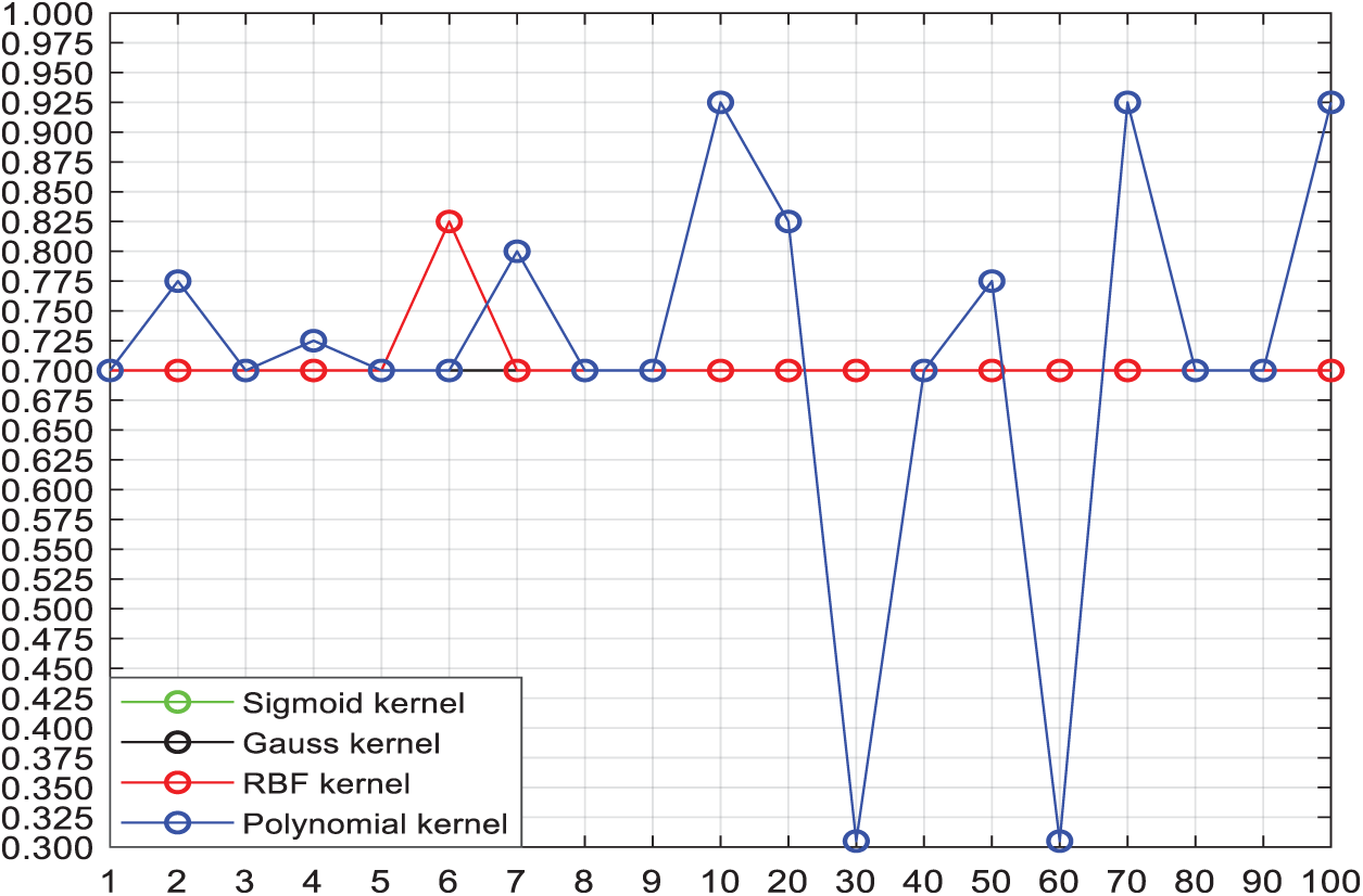
Figure 10: Effect of 4 kinds of kernel functions with different C values on the classification accuracy

Two significantly changed lines in the figure above are RBF [29] kernel and polynomial kernel functions. When C=6 RBF kernel function has a higher accuracy. Its recognition accuracy is independent of the selected σ value. When C=10 and C=70, polynomial kernel function has a relatively high accuracy rate reaching 92.5%. Let the value of C be fixed, and adjust the parameter d of polynomial kernel function to observe the results.

Fig. 11 shows that choosing different kernel parameters in polynomial kernel will result in different effects on the classification accuracy. When C=10, and polynomial kernel parameter d=4, we get the highest classification accuracy, which are adopted to the classification of SVM classifier.

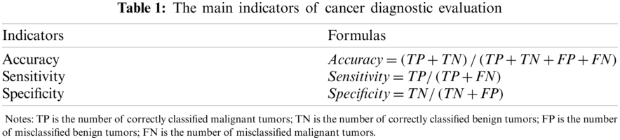
For a diagnosis system, three indicators are doctors’ priority concern, which are accuracy, sensitivity and specificity. Sensitivity reflects the system recognition rate to malignant tumor. The higher sensitivity is, the higher recognition rate to malignant tumor will be. While specificity reflects the system recognition rate to benign tumor. The higher specificity is, the lower rate of benign samples will be wrongly accused of malignant. As defined in Tab. 1.

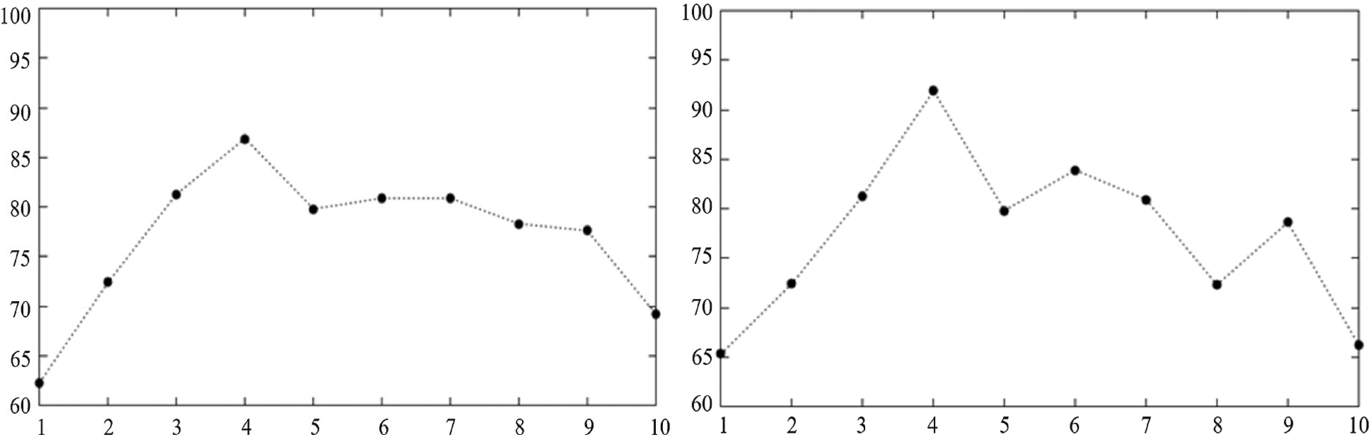
Figure 11: The effect of Polynomial kernel parameters on the classification accuracy when C = 70 and C = 10

The extracted feature vectors are input into different classifiers to analyze and compare the performance of the classification. The experiments of each classifier are conducted 10 times, respectively recording different feature extraction algorithms as well as the average classification performance of the 10 experiments. And referring to the evaluation criteria, accuracy, sensitivity and specificity of the classification results are obtained. The performance comparison among different feature extraction algorithms and different classifiers is shown in Tab. 2.

LBP represents traditional local binary pattern; GLCM (Grey-Level Co-occurrence Matrix) is proposed in [9], which is the feature extraction algorithm based on the gray level co-occurrence matrix of thyroid tumor; FELBP is an updated fuzzy elliptic local binary pattern, improving the coding of neighborhood and distance of LBP; LBP-A-S and FELBP-A-S are fusion feature methods that combine attenuation and shape features on the basis of LBP and FELBP, respectively. It can be seen in Tab. 2 that the proposed method in this paper features the highest classification stability and accuracy under above experimental conditions. Using computer-aided diagnosis aims to improve specificity under 100% sensitivity, ensure all samples in the malignant categories identified as malignant and reduce the situations that benign tumors being mistaken for malignant under the condition that all the malignant samples can be detected. In this way, most of the benign samples would not send to the biopsy, which can reduce the amount of biopsy.

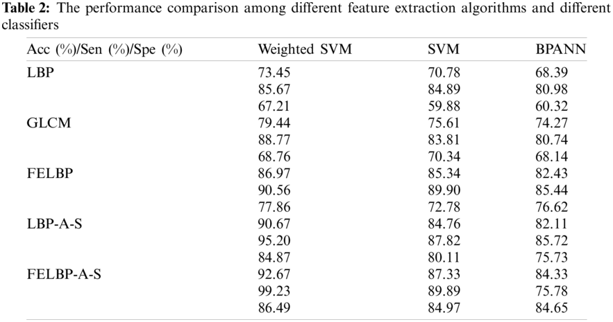
From Tab. 2, we can know that the weighted degree of SVM introduced in this paper efficiently compensate the adverse effect to the classification and prediction accuracy of small class samples caused by unbalanced sample size in each class by giving different classes of samples with different weights. After all, the proposed method has better image segmentation effect, and archive a higher objective evaluation index, and it is worthy to be extended to practical application.

6  Conclusions

Under the research and application background of the ultrasound diagnosis of thyroid nodules, this paper takes the database of thyroid nodules ultrasound images in hospitals as the research object, and combines existing medical conditions with computer technology, image processing technology, artificial intelligence technology and data analysis to process and analyze ultrasound images with computer. Moreover, this paper puts forward an automatic diagnosis system of thyroid nodules based on ultrasound images (TN-CAD). In this system, firstly the level set active contour model of the phase and gradient information is used to complete automatic boundaries extraction of thyroid tumor images, and then a feature extraction algorithm which is specific to thyroid nodule is explored. Finally, an improved support vector machine (SVM) is used for benign and malignant discrimination on thyroid nodules. Experimental results show the effectiveness of the proposed algorithm.

Acknowledgement: Thank you for the supported by the High-Performance Computing Center of Hebei University.

Funding Statement: This work was supported in part by National Natural Science Foundation of China under Grant Nos. 61572063 and 61401308, Natural Science Foundation of Hebei Province under Grant Nos. F2016201142, F2018210148, F2019201151 and F2020201025, Science Research Project of Hebei Province under Grant Nos. BJ2020030, QN2016085 and QN2017306, Foundation of President of Hebei University under Grant No. XZJJ201909, Opening Foundation of Machine Vision Technology Innovation Center of Hebei Province under Grant Nos. 2018HBMV01 and 2018HBMV02, Natural Science Foundation of Hebei University under Grant Nos. 2014-303 and 8012605.

Conflicts of Interest: The authors declare that they have no conflicts of interest to report regarding the present study.

References

 1.  Bozan, M. B., Yazar, F. M., Kale, L. T., Yüzbaşıoğlu, M. F., Boran, O. F. et al. (2020). Delta neutrophil index and neutrophil-to-lymphocyte ratio in the differentiation of thyroid malignancy and nodular goiter. World Journal of Surgery, 45(2), 507–514. DOI 10.1007/s00268-020-05822-6. [Google Scholar] [CrossRef]

 2.  Zheng, Y., Xu, S., Zheng, Z., Wu, L., Chen, L. et al. (2019). Ultrasonic classification of multicategory thyroid nodules based on logistic regression. Ultrasound Quarterly, 36(2), 1. DOI 10.1097/RUQ.0000000000000453. [Google Scholar] [CrossRef]

 3.  Aboudi, N., Guetari, R., Khlifa, N. (2020). Multi-objectives optimization of features selection for the classification of thyroid nodules in ultrasound images. IET Image Processing, 14(9), 1901–1908. DOI 10.1049/iet-ipr.2019.1540. [Google Scholar] [CrossRef]

 4.  Wang, Y., Yue, W., Li, X., Liu, S., Guo, L. et al. (2020). Comparison study of radiomics and deep learning-based methods for thyroid nodules classification using ultrasound images. IEEE Access, 8(3), 52010–52017. DOI 10.1109/ACCESS.2020.2980290. [Google Scholar] [CrossRef]

 5.  Iakovidis, D. K., Keramidas, E. G., Maroulis, D. (2008). Fuzzy local binary patterns for ultrasound texture characterization. International Conference on Image Analysis & Recognition, pp. 11–15, Verlag: Springer. [Google Scholar]

 6.  Chang, C. Y., Chen, S. J., Tsai, M. F. (2010). Application of support-vector-machine-based method for feature selection and classification of thyroid nodules in ultrasound images. Pattern Recognition, 43(10), 3494–3506. DOI 10.1016/j.patcog.2010.04.023. [Google Scholar] [CrossRef]

 7.  Morifuji, H. (1989). Analysis of ultrasound B-mode histogram in thyroid tumors. Nippon Geka Gakkai Zasshi, 90(2), 210–221. DOI 10.2664/1989/9022102. [Google Scholar] [CrossRef]

 8.  Acharya, U. R., Chowriappa, P., Fujita, H., Bhat, S., Dua, S. et al. (2016). Thyroid lesion classification in 242 patient population using Gabor transform features from high resolution ultrasound images. Knowledge-Based Systems, 107(1), 235–245. DOI 10.1016/j.knosys.2016.06.010. [Google Scholar] [CrossRef]

 9.  Xian, G. M. (2010). An identification method of malignant and benign liver tumors from ultrasonography based on GLCM texture features and fuzzy SVM. Expert Systems with Applications, 37(10), 6737–6741. DOI 10.1016/j.eswa.2010.02.067. [Google Scholar] [CrossRef]

10. Shin, Y. G., Yoo, J., Kwon, H. J., Hong, J. H., Lee, H. S. et al. (2016). Histogram and gray level co-occurrence matrix on gray-scale ultrasound images for diagnosing lymphocytic thyroiditis. Computers in Biology & Medicine, 75, 257–266. DOI 10.1016/j.compbiomed.2016.06.014. [Google Scholar] [CrossRef]

11. Mahdi, A., Ravish, J., Ramsha, U., Eraj, H. (2018). Influence of gain settings on strain ratios of elastographic image and texture parameters of B-mode image on thyroid tissue. Biomedical Research, 29(7), 1316–1320. DOI 10.4066/biomedicalresearch.29-17-3994. [Google Scholar] [CrossRef]

12. Savelonas, M. A., Iakovidis, D. K., Dimitropoulos, N., Maroulis, D. (2007). Computational characterization of thyroid tissue in the radon domain. IEEE International Symposium on Computer-Based Medical Systems, 2007, 189–192. DOI 10.1109/CBMS.2007.33. [Google Scholar] [CrossRef]

13. Prabal, P., Alfredo, H., Debdoot, S., Michael, F. (2018). Evaluation of commonly used algorithms for thyroid ultrasound images segmentation and improvement using machine learning approaches. Journal of Healthcare Engineering, 2018, 8087624. DOI 10.1155/2018/8087624. [Google Scholar] [CrossRef]

14. Iakovidis, D. K., Keramidas, E. G., Maroulis, D. (2010). Fusion of fuzzy statistical distributions for classification of thyroid ultrasound patterns. Artificial Intelligence in Medicine, 50(1), 33–41. DOI 10.1016/j.artmed.2010.04.004. [Google Scholar] [CrossRef]

15. Keramidas, E. G., Iakovidis, D. K., Maroulis, D., Dimitropoulos, N. (2008). Thyroid texture representation via noise resistant image features. IEEE International Symposium on Computer-Based Medical Systems, 2008, 560–565. DOI 10.1109/CBMS.2008.108. [Google Scholar] [CrossRef]

16. Fang, L., Wang, X., Wang, L. (2020). Multi-modal medical image segmentation based on vector-valued active contour models. Information Ences, 513, 504–518. DOI 10.1016/j.ins.2019.10.051. [Google Scholar] [CrossRef]

17. Dhara, A. K., Mukhopadhyay, S., Dutta, A., Garg, M., Khandelwal, N. et al. (2016). A combination of shape and texture features for classification of pulmonary nodules in lung CT images. Journal of Digital Imaging, 29(4), 466–475. DOI 10.1007/s10278-015-9857-6. [Google Scholar] [CrossRef]

18. Li, C. M., Xu, C., Gui, C., Fox, M. D. (2010). Distance regularized level set evolution and its application to image segmentation. IEEE Transactions Image Process, 19(12), 3243–3254. DOI 10.1109/TIP.2010.2069690. [Google Scholar] [CrossRef]

19. Wang, S. H., Chen, Y. (2020). Fruit category classification via an eight-layer convolutional neural network with parametric rectified linear unit and dropout technique. Multimedia Tools and Applications, 79(21–22), 15117–15133. DOI 10.1007/s11042-018-6661-6. [Google Scholar] [CrossRef]

20. Wang, D. (2019). Extremely optimized drlse method and its application to image segmentation. IEEE Access, 7(8), 119603–119619. DOI 10.1109/ACCESS.2019.2937512. [Google Scholar] [CrossRef]

21. Morrone, M. C., Owens, R. A. (1987). Feature detection from local energy. Pattern Recognition Letters, 6(5), 303–313. DOI 10.1016/0167-8655(87)90013-4. [Google Scholar] [CrossRef]

22. Wang, S. H., Hong, J., Yang, M. (2020). Sensorineural hearing loss identification via nine-layer convolutional neural network with batch normalization and dropout. Multimedia Tools and Applications, 79(21–22), 15135–15150. DOI 10.1007/s11042-018-6798-3. [Google Scholar] [CrossRef]

23. Wang, S., Jiang, Y., Hou, X., Hong, C., Du, S. (2017). Cerebral micro-bleed detection based on the convolution neural network with rank based average pooling. IEEE Access, 5, 16576–16583. DOI 10.1109/Access.6287639. [Google Scholar] [CrossRef]

24. Tuncer, T., Dogan, S., Ozyurt, F. (2020). An automated residual exemplar local binary pattern and iterative relieff based corona detection method using lung X-ray image. Chemometrics and Intelligent Laboratory Systems, 203, 104054. DOI 10.1016/j.chemolab.2020.104054. [Google Scholar] [CrossRef]

25. Tang, C., Nayak, D. R., Wang, S. (2020). Least-square support vector machine and wavelet selection for hearing loss identification. Computer Modeling in Engineering & Sciences, 125(1), 299–313. DOI 10.32604/cmes.2020.011069. [Google Scholar] [CrossRef]

26. Wang, S., Phillips, P., Liu, A., Du, S. (2017). Tea category identification using computer vision and generalized eigenvalue proximal SVM. Fundamenta Informaticae, 151(1–4), 325–339. DOI 10.3233/FI-2017-1495. [Google Scholar] [CrossRef]

27. Prochazka, A., Gulati, S., Holinka, S., Smutek, D. (2019). Patch-based classification of thyroid nodules in ultrasound images using direction independent features extracted by two-threshold binary decomposition. Computerized Medical Imaging and Graphics, 71(4), 9–18. DOI 10.1016/j.compmedimag.2018.10.001. [Google Scholar] [CrossRef]

28. Laza, R., Pavon, R., Reboiro-Jato, M., Fdez-Riverola, F. (2011). Evaluating the effect of unbalanced data in biomedical document classification. Journal of Integrative Bioinformatics, 8(3), 177–190. DOI 10.1515/jib-2011-177. [Google Scholar] [CrossRef]

29. Wang, S. H., Zhan, T. M., Chen, Y., Zhang, Y., Yang, M. et al. (2016). Multiple sclerosis detection based on biorthogonal wavelet transform, RBF kernel principal component analysis, and logistic regression. IEEE Access, 4, 7567–7576. DOI 10.1109/ACCESS.2016.2620996. [Google Scholar] [CrossRef]

This work is licensed under a Creative Commons Attribution 4.0 International License, which permits unrestricted use, distribution, and reproduction in any medium, provided the original work is properly cited.