Engineering & Sciences
| Computer Modeling in Engineering & Sciences |
DOI: 10.32604/cmes.2021.015807
ARTICLE
ANC: Attention Network for COVID-19 Explainable Diagnosis Based on Convolutional Block Attention Module
1Jiangsu Key Laboratory of Advanced Manufacturing Technology, Huaiyin Institute of Technology, Huai’an, 223003, China
2Department of Medical Imaging, The Fourth People’s Hospital of Huai’an, Huai’an, 223002, China
3School of Informatics, University of Leicester, Leicester, LE1 7RH, UK
*Corresponding Authors: Yudong Zhang. Email: yudongzhang@ieee.org; Xin Zhang. Email: hasyzx@njmu.edu.cn
Received: 15 January 2021; Accepted: 24 February 2021
Abstract: Aim: To diagnose COVID-19 more efficiently and more correctly, this study proposed a novel attention network for COVID-19 (ANC). Methods: Two datasets were used in this study. An 18-way data augmentation was proposed to avoid overfitting. Then, convolutional block attention module (CBAM) was integrated to our model, the structure of which is fine-tuned. Finally, Grad-CAM was used to provide an explainable diagnosis. Results: The accuracy of our ANC methods on two datasets are
Keywords: Deep learning; convolutional block attention module; attention mechanism; COVID-19; explainable diagnosis
COVID-19 (also known as coronavirus) pandemic is an ongoing infectious disease [1] caused by severe acute respiratory syndrome (SARS) coronavirus 2 [2]. As of 7/Feb/2021, there are over 106.22 m confirmed cases and over 2.31 m deaths attributed to COVID-19 (See Fig. 1). The main symptoms of COVID-19 are a low fever, a new and ongoing cough, a loss or change to taste and smell [3].
In UK, the vaccines approved were developed by Pfizer/BioNTech, Oxford/AstraZeneca, and Moderna [4]. The joint committee on vaccination and immunization (JCVI) [5] determines the order in which people will be offered the vaccine. Currently, people aged over 80, people living or working in the care homes, and health care providers are being offered.
Two COVID-19 diagnosis methods are available. The first method is viral testing to test the existance of viral RNA fragments [6]. The shortcomings are two folds: (i) the swab may be contaminated and (ii) it needs to wait from several hours to several days to get the results. The other method is chest imaging. The chest computed tomography (CCT) [7] is one of the best chest imaging techniques. CCT is operator independent. Besides, it provides the highest sensitivity compared to ultrasound and X-ray [8]. It provides real 3D volumetric image of the chest region [9].

Figure 1: The cumulative data till 7/Feb/2021. (a) Cumulative cases, (b) cumulative deaths
Nevertheless, the manual labelling by human experts are time-consuming, tedious, labor-intensive, and easily influenced by human factors (fatiguing or lethargic emotions). In contrast to manual labelling, computer vision techniques [10] are now gaining promising results on automatic labelling of COVID-19 and other medical images with the help of artificial intelligence (AI) [11].
For non-COVID-19 images, Lu [12] proposed a bat algorithm-based extreme learning machine (BA-ELM) approach, and applied it to pathological brain detection. Lu [13] presented a radial basis function (RBFNN) to recognize pathological brain types. Fulton et al. [14] employed ResNet-50 for identifying Alzheimer’s disease. Guo et al. [15] utilized ResNet-18 to identify Thyroid ultrasound plane images. Although those above methods were not directly developed for COVID-19 diagnosis, they are chosen and used as comparison methods in this study.
For COVID-19 images, Yu [16] proposed GoogleNet-COD model. The authors first replaced the last two layers with four new layers, which included the dropout layer, two fully connected layers and the output layer. Satapathy [17] proposed a five-layer deep convolutional neural network with stochastic pooling (DCNN-SP). Yao [18] combined wavelet entropy (WE) and biogeography-based optimization (BBO) techniques. Wu [19] used wavelet Renyi entropy (WRE) to extract features from chest CT images. Li et al. [20] presented a COVID-19 detection neural network (COVNet). Akram et al. [21] proposed a four-step procedure to handle COVID-19: (i) data collection & normalization; (ii) feature extraction; (iii) feature selection;, and (iv) feature classification. Khan et al. [22] used one class kernel extreme learning machine to predict COVID-19 pneumonia. Khan et al. [23] used DenseNet and firefly algorithm for classification of positive COVID-19 CT scans.
To further improve the COVID-19 diagnosis performance, this paper proved a novel AI model, attention network for COVID (ANC), for providing an explainable diagnosis. Here “attention” means it can tell neural network which region should focus. Compared to ordinary neural networks, the advantages of ANC are four folds:
i) A novel 18-way data augmentation was proposed to avoid overfitting;
ii) Convolutional block attention module was integrated so our model can infer attention maps;
iii) Our model was fine-tuned, and its performances were better than 9 state-of-the-art approaches;
iv) Grad-CAM was used to provide an explainable heatmap so the users can understand our model.
Two datasets are used in this study. The first dataset contains 148 COVID-19 images and 148 healthy control (HC) images [19]. The second dataset contains 320 COVID-19 images and 320 HC images [24]. Tab. 1 provides the descriptions of these two COVID-19 CCT datasets, where a + b stands for a COVID-19 subject/images and b HC subjects/images.
Table 1: Descriptions of two COVID-19 CCT datasets

Preprocessing were applied to all the images. Let R0 and R stand for the raw dataset ( Dataset-1 or Dataset-2) and the final preprocessed set, and R1, R2, R3 denote three temporary sets. The flowchart of our pre-processing is displayed in Fig. 2.
Th raw dataset set

Figure 2: Flowchart of preprocessing
First, we need to grayscale all those raw images. The grayscale transformation is described as
which utilized the standard RGB to grayscale transformation [25].
Second, the histogram stretching (HS) was used to improve the contrast of all grayscaled images
where
The new HS-enhanced image
where
The HS-enhanced image will occupy the full grayscale range as
Third, we cropped the texts at the right region and the check-up bed at the bottom region. The crop values
where
where
Finally, downsampling was carried out to further reduce the image size and remove redundant information. Suppose the final size is
where fds is the downsampling function defined as
Figs. 3a and 3b show the raw and pre-processed images of a COVID-19 case, while Figs. 3c and 3d illustrates the raw and pre-processed images of a HC case. As can be observed from Fig. 3, the pre-processed images have better contrast, remove the irrelevant information, down-sample to a smaller size, and take less storage than the raw images. Tab. 2 itemizes the abbreviation list, which will help readers to understand the following sections.

Figure 3: Raw images and pre-processed images selected from our datasets. (a) Raw COVID-19 image, (b) pre-processed image of (a), (c) raw HC image, (d) pre-processed image of (c)

Data augmentation (DA) is an important tool over the training set to avoid overfitting of classifiers, and to overcome the small-size dataset problem. Recently, Wang [26] proposed a novel 14-way data augmentation (DA), which used seven different DA techniques to the preprocessed image
This study enhances the 14-way DA method [26] to 18-way DA, by adding two new DA methods: salt-and-pepper noise (SAPN) and speckle noise (SN) on both

Figure 4: Illustration of two new DAs. (a) Raw image, (b) SAPN altered, (c) SN altered
For a given image
where
On the other side, the SN altered image [28] is defined as
where
Let Na stands for the number of DA techniques to the preprocessed image
First, Na geometric/photometric/noise-injection DA transforms are utilized on preprocessed image

Figure 5: Schematic of proposed 18-way DA
Second, horizontal mirror image is generated as
where hM means horizontal mirror function.
Third, all the Na different DA methods are carried out on the mirror image
Four, the raw image
The final combined dataset is defined as
Therefore, one image
images (including the original image

3.2 Convolutional Block Attention Module
Deep learning (DL) has gained successes in prediction/classification tasks. There are many DL structures, such as deep neural network [29], deep belief network, convolutional neural network (CNN) [30], recurrent neural network [31], graph neural network, etc. Among all those DL structures, CNN is particularly suitable for analyzing visual images.
To further improve the performance of CNN, a lot of researches are done with respects to either depth, or width, or cardinality of CNN. In recent times, Woo et al. [32] proposed a novel convolutional block attention module (CBAM), which improves the traditional convolutional block (CB) by integrating attention mechanism. There are many successful applications of CBAM. For example, Mo et al. [33] combined self-attention and CBAM. They proposed a light-weight dual-path attention block. Chen et al. [34] proposed a 3D spatiotemporal convolutional neural network with CBAM for micro-expression recognition.
Fig. 6a displays the structure of a traditional CB. The output of previous block was sent to n-repetitions of convolution layer, batch normalization (BN), rectified linear unit (ReLU) layer, and followed by a pooling layer. The output is called activation map (AM), symbolized as

Figure 6: Structural comparison with CB against CBAM. (a) Traditional CB, (b) our CBAM
In contrast to Figs. 6a and 6b displays the structure of CBAM, in which two modules: channel attention module (CAM) and spatial attention module (SAM) are added to refine the activation map
And the final refined AM
where
Note if the two operands are not with the same dimension, then the values are broadcasted (copied) in such ways the spatial attentional values are broadcasted along the channel dimension, and the channel attention values are broadcasted along the spatial dimension.
We define the CAM here. Both max pooling (MP) [35] zmp and average pooling (AP) [36] zmp are utilized, generating two features
Both
To reduce the parameter resources, the hidden size of MLP is set to
Note

Figure 7: Flowchart of CAM
Now we define the spatial attention module (SAM) as shown in Fig. 8. The spatial attention module
Both

Figure 8: Flowchart of SAM
The concatenated activation map is then passed into a standard
The
3.5 Proposed Attention Network for COVID-19
In this study, we proposed a novel Attention Network for COVID-19 (ANC) based on CBAM (See Fig. 6b). The structure of this proposed ANC is determined by trial-and-error method. The variable n in each block varies, and we found the best values are chosen in the range from
The structure of proposed shown below in Tab. 3, which is a 15-layer deep CNN. The Input I is a
Table 3: Structure of proposed ANC

Here T5 is used to generate heatmap by the gradient-weighted class activation mapping (Grad-CAM) [38] method, which shows explanations (i.e., heatmaps) which region the ANC model pays more attention to and how our ANC model makes prediction.
The variable FL is then sent to three consecutive fully-connected layers (FCLs). The neurons of those three FCLs are set to 200, 50, and 2, respectively. The output of those three FCLs are symbolized as F1, F2, and F3, respectively, as shown in Fig. 9. Finally, F3 is sent through a softmax layer to output the probabilities of all classes.

Figure 9: Variables and sizes of AMs of proposed ANC
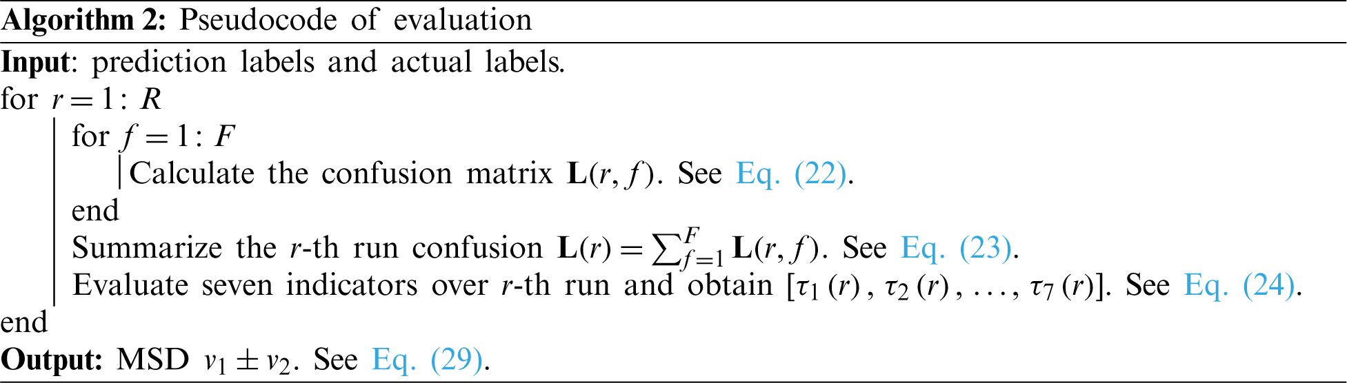
3.6 Implementation and Evaluation
F-fold cross validation is employed on both datasets. Suppose confusion matrix
where

Figure 10: Diagram of one run of F-fold cross validation
Note that
Seven indicators
where first four indicators are:
and
There are two indicators
Above procedure is one run of F-fold cross validation. In the experiment, we run the F-fold cross validation R runs. The mean and standard deviation (MSD) of all seven indicators
where v1 stands for the mean value, and v2 stands for the standard deviation. The MSDs are reported in the format of
4 Experiments, Results, and Discussions
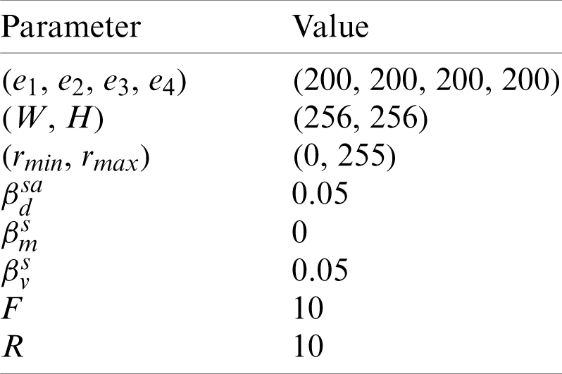
Tab. 4 shows the parameter setting. Here the crop values of top, bottom, left, and right are all set to 200 pixels. The size of preprocessed image is set to

Figure 11: Na DA results on original preprocessed image. (a) Gaussian noise, (b) SAPN, (c) SN, (d) horizontal shear, (e) vertical shear, (f) rotation, (g) gamma correction, (h) random translation, (i) scaling
4.2 Results of Proposed 18-Way DA
Take Fig. 3b as an example, Fig. 11 displays the Na results of this original image. Due to the page limit, the horizontal mirrored image and its corresponding Na results are not displayed in Fig. 11. As it is calculated, one image will generate
4.3 Statistics of Proposed ANC
First, the statistical results on the first dataset and the second dataset are shown in Tabs. 5 and 6 respectively. We can observe that for Dataset-1, the sensitivity is
Table 5: Statistical results of proposed ANC model on D1
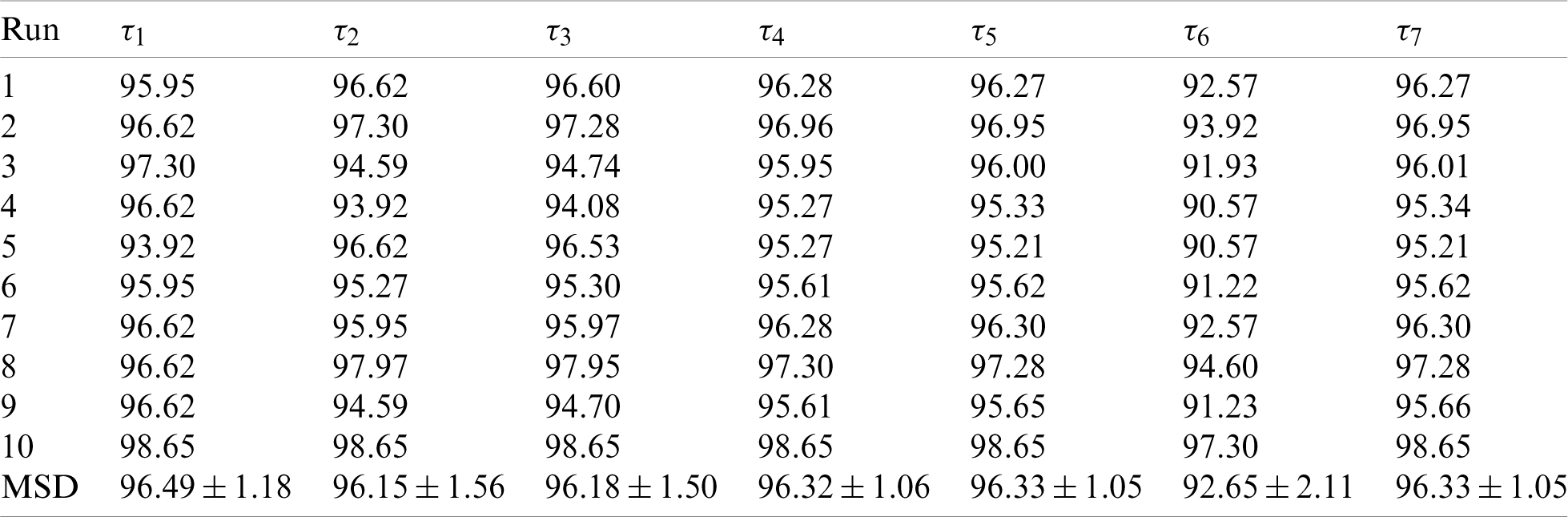
Table 6: Statistical results of proposed ANC model on D2
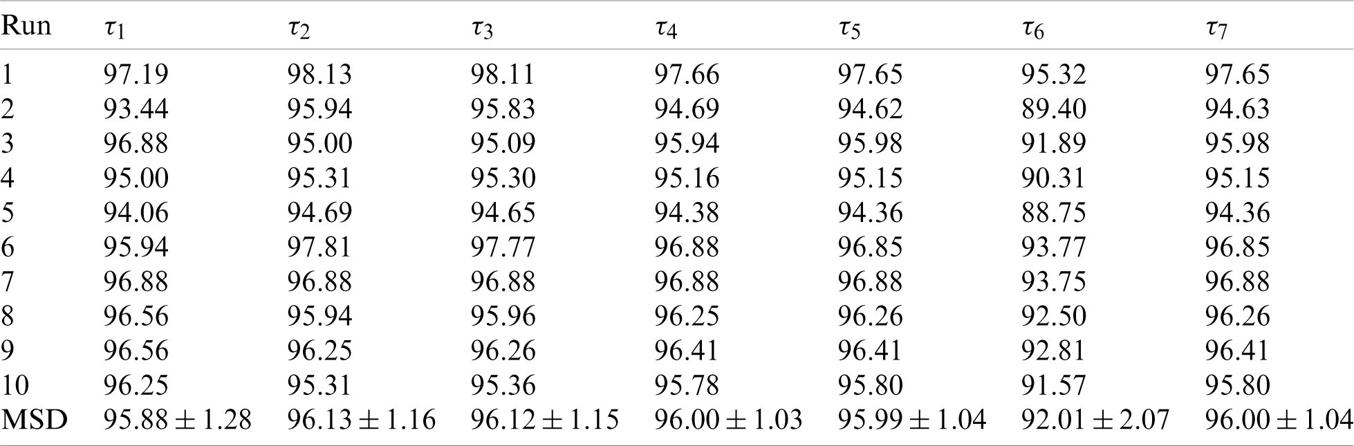

Figure 12: ROC curves of proposed ANC model (10 runs). (a) Dataset D1 (
4.4 Effect of Attention Mechanism
This ablation study removed attention blocks (CAM and SAM) from our ANC model. Here NA in Tab. 7 means no attention. Tab. 7 shows that removing attention blocks will reduce the performance significantly. For example, the MCCs, i.e.,
Fig. 13 shows the error bars of different models, where D1 and D2 stand for the 1st and 2nd dataset, respectively, as introduced in Section 2. It clearly indicates that using attention mechanism can help improve the classification performances on both datasets.
Table 7: Comparison of models with attention against without attention
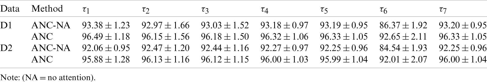

Figure 13: Effect of attention mechanism on two datasets. (D1: the first dataset; D2: the second dataset)
4.5 Comparison to State-of-the-Art Approaches
We compare our method “ANC” with 9 state-of-the-art methods: ELM-BA [12], RBFNN [13], ResNet-50 [14], ResNet-18 [15], GoogleNet-COD [16], DCNN-SP [17], WE-BBO [18], WRE [19], and COVNet [20]. All the methods were evaluated via 10 runs of 10-fold cross validation. The MSD results
Table 8: Comparison with SOTA approaches in two datasets (unit: %)
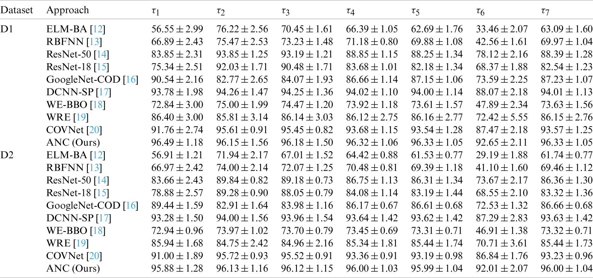

Figure 14: Comparison to state-of-the-art approaches over two datasets (D1 and D2). (a) D1, (b) D2

Figure 15: Manual delineation and heatmap results of COVID-19 sample image. (a) Manual delineation of COVID-19, (b) heatmap of (a), (c) HC image, (d) heatmap of (c)
Fig. 14 shows the 3D bar plot of our ANC method and 9 state-of-the-art algorithms. All the algorithms are sorted in terms of
Fig. 15 shows the manual delineation and heatmap results of Fig. 3. Figs. 15a–15c show the delineation, where the healthy control image has no lesion (Fig. 15c), so the radiologist does not delineate the lesion regions in Fig. 15c. Figs. 15b–15d show the corresponding heatmaps, where we can observe that this proposed ANC model can find the COVID-19 related regions correctly.
This paper proposed a novel attention network for COVID-19 (ANC) model. The classification results of ANC model are better than 9 state-of-the-art approaches in terms of seven indicators: sensitivity, specificity, precision, accuracy, F1 score, MCC, and FMI.
There are two disadvantages of our proposed method: (i) The dataset is relatively small. We expect to expand the dataset to have more than 1k images. (ii) Graph neural network technologies will be attempted to integrate to our model.
Funding Statement: This paper is partially supported by Open Fund for Jiangsu Key Laboratory of Advanced Manufacturing Technology (HGAMTL-1703); Guangxi Key Laboratory of Trusted Software (kx201901); Fundamental Research Funds for the Central Universities (CDLS-2020-03); Key Laboratory of Child Development and Learning Science (Southeast University), Ministry of Education; Royal Society International Exchanges Cost Share Award, UK (RP202G0230); Medical Research Council Confidence in Concept Award, UK (MC_PC_17171); Hope Foundation for Cancer Research, UK (RM60G0680); British Heart Foundation Accelerator Award, UK.
Conflicts of Interest: The authors declare that they have no conflicts of interest to report regarding the present study.
1. Rauf, H. T., Lali, M. I. U., Khan, M. A., Kadry, S., Alolaiyan, H. et al. (2021). Time series forecasting of COVID-19 transmission in Asia Pacific countries using deep neural networks. Personal and Ubiquitous Computing, 9(3), 674. DOI 10.1007/s00779-020-01494-0. [Google Scholar] [CrossRef]
2. Marquez, R., Tolosa, L., Celis, M. T. (2021). Understanding COVID-19 effect on the U.S. supply chain of strategic products: Important factors, current situation, and future perspective. Revista Ciencia e Ingenier¡́x0131/¿a, 42(1), 53–62. http://erevistas.saber.ula.ve/index.php/cienciaeingenieria/article/viewFile/16645/21921927789. [Google Scholar]
3. Avci, H., Karabulut, B. (2021). The relation between otolaryngology-specific symptoms and computed tomography findings in ambulatory care COVID-19 patients. Ear Nose Throat Journal, 100(2), 79–85. DOI 10.1177/0145561320975508. [Google Scholar] [CrossRef]
4. Mahase, E. (2021). Covid-19: UK approves moderna vaccine to be given as two doses 28 days apart. British Medical Journal, 372, 1. DOI 10.1136/bmj.n74. [Google Scholar] [CrossRef]
5. Hall, A. J. (2010). The United Kingdom joint committee on vaccination and immunisation. Vaccine, 28, 54–57. DOI 10.1016/j.vaccine.2010.02.034. [Google Scholar] [CrossRef]
6. Goncalves, J., Koritnik, T., Mioc, V., Trkov, M., Boljesic, M. et al. (2021). Detection of SARS-CoV-2 RNA in hospital wastewater from a low COVID-19 disease prevalence area. Science of the Total Environment, 755, 7. DOI 10.1016/j.scitotenv.2020.143226. [Google Scholar] [CrossRef]
7. Teichgraber, U., Malouhi, A., Ingwersen, M., Neumann, R., Reljic, M. et al. (2021). Ruling out COVID-19 by chest CT at emergency admission when prevalence is low: The prospective, observational SCOUT study. Respiratory Research, 22(1), 11. DOI 10.1186/s12931-020-01611-w. [Google Scholar] [CrossRef]
8. Nayak, S. R., Nayak, D. R., Sinha, U., Arora, V., Pachori, R. B. (2021). Application of deep learning techniques for detection of COVID-19 cases using chest X-ray images: A comprehensive study. Biomedical Signal Processing and Control, 64, 12. DOI 10.1016/j.bspc.2020.102365. [Google Scholar] [CrossRef]
9. Leonard-Lorant, I., Severac, F., Bilbault, P., Muller, J., Leyendecker, P. et al. (2021). Normal chest CT in 1091 symptomatic patients with confirmed COVID-19: Frequency, characteristics and outcome. European Radiology, 6, pp. 1–6. DOI 10.1007/s00330–020-07593-z. [Google Scholar] [CrossRef]
10. Khemasuwan, D., Sorensen, J. S., Colt, H. G. (2020). Artificial intelligence in pulmonary medicine: Computer vision, predictive model and COVID-19. European Respiratory Review, 29(157), 16. DOI 10.1183/16000617.0181-2020. [Google Scholar] [CrossRef]
11. Kabra, R., Singh, S. (2021). Evolutionary artificial intelligence based peptide discoveries for effective COVID-19 therapeutics. Biochimica et Biophysica Acta (BBA)—Molecular Basis of Disease, 1867(1), 13. DOI 10.1016/j.bbadis.2020.165978. [Google Scholar] [CrossRef]
12. Lu, S. (2017). A pathological brain detection system based on extreme learning machine optimized by bat algorithm. CNS & Neurological Disorders-Drug Targets, 16(1), 23–29. DOI http://dx.doi.org/10.2174/1871527315666161019153259. [Google Scholar]
13. Lu, Z. (2016). A pathological brain detection system based on radial basis function neural network. Journal of Medical Imaging and Health Informatics, 6(5), 1218–1222. DOI 10.1166/jmihi.2016.1901. [Google Scholar] [CrossRef]
14. Fulton, L. V., Dolezel, D., Harrop, J., Yan, Y., Fulton, C. P. (2019). Classification of Alzheimer’s disease with and without imagery using gradient boosted machines and ResNet-50. Brain Sciences, 9(9), Article ID: 212. DOI 10.3390/brainsci9090212. [Google Scholar] [CrossRef]
15. Guo, M. H., Du, Y. Z. (2019). Classification of thyroid ultrasound standard plane images using ResNet-18 networks. IEEE 13th International Conference on Anti-Counterfeiting, Security, and Identification, Proceedings of the International Conference on Anti-counterfeiting Security and Identification, pp. 324–328. Xiamen, China. [Google Scholar]
16. Yu, X. (2020). Detection of COVID-19 by GoogLeNet-COD. Lecture Notes in Computer Science, 12463, 499–509. DOI 10.1007/978-3-030-60799-9_43. [Google Scholar] [CrossRef]
17. Satapathy, S. C. (2021). A five-layer deep convolutional neural network with stochastic pooling for chest CT-based COVID-19 diagnosis. Machine Vision and Applications, 32. [Google Scholar]
18. Yao, X. (2020). COVID-19 Detection via wavelet entropy and biogeography-based optimization. In: Santosh, K. C., Joshi, A. (Eds.COVID-19: Prediction, decision-making, and its impacts, pp. 69–76. Berlin/Heidelberg, Germany: Springer. [Google Scholar]
19. Wu, X. (2020). Diagnosis of COVID-19 by wavelet Renyi entropy and three-segment biogeography-based optimization. International Journal of Computational Intelligence Systems, 13(1), 1332–1344. DOI 10.2991/ijcis.d.200828.001. [Google Scholar] [CrossRef]
20. Li, L., Qin, L., Xu, Z., Yin, Y., Wang, X. et al. (2020). Using artificial intelligence to detect COVID-19 and community-acquired pneumonia based on pulmonary CT: Evaluation of the diagnostic accuracy. Radiology, 296(2), E65–E71. DOI 10.1148/radiol.2020200905. [Google Scholar] [CrossRef]
21. Akram, T., Attique, M., Gul, S., Shahzad, A., Altaf, M. et al. (2021). A novel framework for rapid diagnosis of COVID-19 on computed tomography scans. Pattern Analysis and Applications, 382(2), 727. DOI 10.1007/s10044-020-00950-0. [Google Scholar] [CrossRef]
22. Khan, M. A., Kadry, S., Zhang, Y. D., Akram, T., Sharif, M. et al. (2021). Prediction of COVID-19-pneumonia based on selected deep features and one class kernel extreme learning machine. Computers & Electrical Engineering, 90, 106960. DOI 10.1016/j.compeleceng.2020.106960. [Google Scholar] [CrossRef]
23. Khan, M. A., Hussain, N., Majid, A., Alhaisoni, M., Bukhari, S. A. C. et al. (2021). Classification of positive COVID-19 CT scans using deep learning. Computers, Materials & Continua, 66(3), 2923–2938. DOI 10.32604/cmc.2021.013191. [Google Scholar] [CrossRef]
24. Zhang, Y. D. (2020). A seven-layer convolutional neural network for chest CT based COVID-19 diagnosis using stochastic pooling. IEEE Sensors Journal, DOI 10.1109/JSEN.2020.3025855. [Google Scholar] [CrossRef]
25. Sowmya, V., Govind, D., Soman, K. P. (2017). Significance of contrast and structure features for an improved color image classification system. 2017 IEEE International Conference on Signal and Image Processing Applications. pp. 210–215. Kuching, Malaysia. [Google Scholar]
26. Wang, S. H. (2021). Covid-19 classification by FGCNet with deep feature fusion from graph convolutional network and convolutional neural network. Information Fusion, 67, 208–229. DOI 10.1016/j.inffus.2020.10.004. [Google Scholar] [CrossRef]
27. Sagar, P., Upadhyaya, A., Mishra, S. K., Pandey, R. N., Sahu, S. S. et al. (2020). A circular adaptive median filter for salt and pepper noise suppression from MRI images. Journal of Scientific and Industrial Research, 79(10), 941–944. http://nopr.niscair.res.in/handle/123456789/55470. [Google Scholar]
28. Karimi, N., Taban, M. R. (2021). A convex variational method for super resolution of SAR image with speckle noise. Signal Processing-Image Communication, 90, 11. DOI 10.1016/j.image.2020.116061. [Google Scholar] [CrossRef]
29. Jeong, Y., Lee, B., Han, J. H., Oh, J. (2021). Ocular axial length prediction based on visual interpretation of retinal fundus images via deep neural network. IEEE Journal of Selected Topics in Quantum Electronics, 27(4), 7. DOI 10.1109/jstqe.2020.3038845. [Google Scholar] [CrossRef]
30. Lee, Y. Y., Halim, Z. A. (2020). Stochastic computing in convolutional neural network implementation: A review. PeerJ Computer Science, 35, Article ID: e309. DOI 10.7717/peerj–cs.309. [Google Scholar] [CrossRef]
31. Hassan, A. A., El-Habrouk, M., Deghedie, S. (2020). Inverse kinematics of redundant manipulators formulated as quadratic programming optimization problem solved using recurrent neural networks: A review. Robotica, 38(8), 1495–1512. DOI 10.1017/s0263574719001590. [Google Scholar] [CrossRef]
32. Woo, S., Park, J., Lee, J. Y., Kweon, I. S. (2018). CBAM: Convolutional block attention module. Proceedings of the European Conference on Computer Vision. pp. 3–19. Munich, Germany: Springer. [Google Scholar]
33. Mo, J. Y., Xu, L. (2020). Weighted cluster-range loss and criticality-enhancement loss for speaker recognition. Applied Sciences—Basel, 10(24), 20. DOI 10.3390/app10249004. [Google Scholar] [CrossRef]
34. Chen, B. Y., Zhang, Z. H., Liu, N., Tan, Y., Liu, X. et al. (2020). Spatiotemporal convolutional neural network with convolutional block attention module for micro-expression recognition. Information-an International Interdisciplinary Journal, 11(8), 14. DOI 10.3390/info11080380. [Google Scholar] [CrossRef]
35. Akbas, G. E., Kozubek, M. (2020). Condensed U-Net (CU-NetAn improved u-net architecture for cell segmentation powered by
36. Kumar, R. L., Kakarla, J., Isunuri, B. V., Singh, M. (2021). Multi-class brain tumor classification using residual network and global average pooling. Multimedia Tools and Applications, 10, DOI 10.1007/s11042-020-10335-4. [Google Scholar] [CrossRef]
37. Hu, J., Shen, L., Albanie, S., Sun, G., Wu, E. H. (2020). Squeeze-and-excitation networks. IEEE Transactions on Pattern Analysis and Machine Intelligence, 42(8), 2011–2023. DOI 10.1109/TPAMI.2019.2913372. [Google Scholar] [CrossRef]
38. Selvaraju, R. R., Cogswell, M., Das, A., Vedantam, R., Parikh, D. et al. (2020). Grad-CAM: Visual explanations from deep networks via gradient-based localization. International Journal of Computer Vision, 128(2), 336–359. DOI 10.1007/s11263-019-01228-7. [Google Scholar] [CrossRef]
 | This work is licensed under a Creative Commons Attribution 4.0 International License, which permits unrestricted use, distribution, and reproduction in any medium, provided the original work is properly cited. |