Computer Modeling in Engineering & Sciences

DOI: 10.32604/cmes.2021.015688

ARTICLE

Topology and Shape Optimization of 2-D and 3-D Micro-Architectured Thermoelastic Metamaterials Using a Parametric Level Set Method

Ellie Vineyard1 and Xin-Lin Gao2,*

1PepsiCo R&D Center, Valhalla, NY 10595, USA
2Department of Mechanical Engineering, Southern Methodist University, Dallas, TX 75275-0337, USA
*Corresponding Author: Xin-Lin Gao. Email: xlgao@smu.edu
Received: 05 January 2021; Accepted: 24 February 2021

1  Introduction

Micro-architectured thermoelastic metamaterials are a new class of materials with unusual thermal and elastic properties such as a negative Poisson’s ratio and a non-positive coefficient of thermal expansion (CTE) (e.g., [1–7]). For such metamaterials, micro-architectures play a crucial role in attaining targeted or extremal properties beyond those of their constituents. It offers additional degrees of freedom to achieve exotic properties that are not exhibited by naturally occurring or conventionally designed materials.

In developing these metamaterials, heuristic approaches have typically been used (e.g., [1,8–14]). However, such approaches are limited to simple geometrical designs or loading conditions. For complex configurations and deformation mechanisms, topology optimization has emerged as a promising method (e.g., [15–18]). Sigmund et al. [19,20] optimally designed materials with a zero or negative CTE based on the solid isotropic material with penalization (SIMP) method. They found that materials with a negative CTE can be obtained by using two solid materials (each having a positive CTE) and one void phase. Schwerdtfeger et al. [21] optimized a 3-D structure with a negative Poisson’s ratio and increased the negativity of Poisson’s ratio by a factor 2 using a SIMP based inverse homogenization approach. Andreassen et al. [22] designed a manufacturable 3-D elastic microstructure with a Poisson’s ratio of −0.5 through topology optimization with a manufacturing constraint. Wang et al. [23] proposed multi-phase metamaterials with unusual thermoelastic properties by using a parametric level set-based topology optimization method combined with a finite element approach. Vogiatzis et al. [24] employed a reconciled level set-based topology optimization method to design single- and multiple-phase metamaterials with negative Poisson’s ratios in both 2-D and 3-D configurations. Takezawa et al. [25] developed a topology optimization method for porous composites with anisotropic negative CTEs and isotropic/anisotropic positive CTEs. Wang et al. [26] designed multi-phase and multi-functional metamaterials with targeted effective elastic moduli and CTEs and proposed some periodic microstructures that can produce negative Poisson’s ratios and negative CTEs. Ye et al. [27] developed an optimization framework for gradually stiffer mechanical metamaterials with a negative Poisson’s ratio using a parametric level set method and a numerical homogenization approach. Li et al. [28] proposed a robust topology optimization model for thermoelastic properties of multiphase metamaterials by considering hybrid interval-random uncertainties in properties of constituent materials. However, these authors did not consider 3-D cases or anisotropic CTEs under constraints of Poisson’s ratio varying from negative to positive values. This motivated the current study.

In the present paper, topology optimization of micro-architectured multiphase thermoelastic metamaterials is conducted using a parametric level set method combined with a finite element analysis. The -constraint multi-objective optimization method is adopted. An asymptotic homogenization approach is employed to obtain the effective thermoelastic properties of the metamaterials, and the method of moving asymptotes is applied to solve the optimization problem. Both 2-D and 3-D design examples are included to illustrate the new approach, which differs from what was done in [20,26] and other existing studies on topology optimization of multiphase metamaterials with extreme thermoelastic properties, where only 2D configurations were considered in their design examples. In Section 2, the asymptotic homogenization method for predicting effective thermoelastic properties of composites is briefly introduced. Existing analytical formulas for bounds on the effective CTE of heterogeneous composites are reviewed in Section 3. In Section 4, the topology optimization based on the parametric level set method (PLSM) is formulated, which is followed by a sensitivity analysis in Section 5. Numerical results for 2-D and 3-D design examples are presented in Section 6. The paper concludes in Section 7 with a summary.

2  Asymptotic Homogenization of Thermoelastic Properties

Asymptotic homogenization is a widely used approach in which two spatial scales (i.e., microscopic and macroscopic) are considered (e.g., [29–31]). The coordinate system at the microscopic scale is , while that at the macroscopic scale is . The two scales are linked through , where ( > 0) is a small dimensionless parameter.

Using the double-scale asymptotic expansion, the displacement field in a periodic heterogeneous (composite) material can be expressed as

(1)

where (i = 1, 2, 3) denote the homogeneous parts, and (i = 1, 2, 3; k = 1, 2, 3,) represent local variations at the scale of heterogeneities. Note that is periodic in y (also known as Y-periodic), i.e., for any integers n1, n2 and n3 and periods Y1, Y2 and Y3.

It then follows from Eq. (1) that the derivative of the displacement field with respect to the macroscopic coordinate x can be obtained as, with the help of the chain rule and the relation ,

(2)

In addition, the limit of the integral of a Y-periodic function as approaches zero is given by (e.g., [29])

(3)

where is the domain occupied by the material, Y represents a unit cell of the material, and is the unit cell area (in a 2-D case) or volume (in a 3-D case).

According to the principle of virtual work, the equilibrium equation of a material undergoing thermoelastic deformations can be written as (e.g., [29,32])

(4)

where is the material domain with microstructures, is the traction-prescribed part of the smooth closed boundary surface of , is the interface (or hole surface), Cijkl are the components of the elasticity (stiffness) tensor, vi are the components of the virtual displacement, bi are the components of the body force, ti are the components of the traction on the boundary part , pi are the components of the traction on the interface , and is the temperature change.

Using Eqs. (2) and (3) in Eq. (4) gives the following three hierarchical equations based on the order of (e.g., [32]):

(5)

(6)

(7)

where , and are, respectively, the effective (homogenized) elastic stiffness, thermal stress and coefficient of thermal expansion tensors, and are, respectively, the characteristic displacement fields induced by the mechanical and thermal loading, which can be obtained from (e.g., [20])

(8)

(9)

Note that Eqs. (5) and (6) can each be rewritten in a symmetric form as (e.g., [20,33])

(10)

(11)

where stands for three or six linearly independent unit test strain fields for the 2-D or 3-D case, and and represent the locally varying strain and thermal strain fields induced, respectively, by the test strain modes and thermal load, which can be obtained from

(12)

(13)

Also, Eqs. (8) and (9) can be rewritten as, with the help of Eqs. (12) and (13) and the symmetry of Cijkl,

(14)

(15)

3  Bounds on the Effective Coefficient of Thermal Expansion

Several analytical and semi-analytical formulas have been provided to evaluate the effective CTE of heterogeneous composites, which include those reported in [34–37]. The model by Gibiansky et al. [37], which gives tight and sharp bounds compared to those presented in Schapery [35] and Rosen et al. [36], is adopted in this study. The upper and lower bounds on the effective CTE read [20,37]

(16a)

for 2-D cases, where

(16b)

and

(17a)

for 3-D cases, where

(17b)

In Eqs. (16a), (16b), (17a) and (17b), represents the volume average of the property for the multi-phase composite, with vfn being the volume fraction of each phase and N the number of phases, and are, respectively, the minimum and maximum shear moduli, and are the lower and upper Hashin-Shtrikman bounds on the 2-D bulk modulus given by [20,38]

(18a)

(18b)

and and are, respectively, the lower and upper Hashin-Shtrikman bounds on the 3-D bulk modulus given by [38,39]

(19a)

(19b)

where for the 2-D plane stress case and for the 3-D case, and for both the 2-D and 3-D cases (e.g., [40]).

4  Topology Optimization Using the PLSM

The parametric level set method (PLSM) developed in [41,42] is a powerful shape and topology optimization approach that can overcome some shortcomings of the conventional level set method, such as no regularization, velocity extension, and numerical time step limitations (e.g., [43]). In addition, for multi-material optimizations, Wang et al. [44] proposed the use of m level set functions to conduct multi-phase structural optimizations on the basis of the PLSM, which can prevent overlapping between different phases and suppress redundant regions in the design domain when compared to other multi-material approaches (e.g., [45,46]).

In order to obtain multi-functional composites with optimal properties, multi-objective topology optimization methods need to be used. A few algorithms have been developed to achieve multi-objective optimization. The weighted sum optimization method is a classical approach that combines all the objectives into a single objective function, where the designer prescribes the weights a priori. Different weights can be assigned to different terms in the objective function based on their relative importance. These weights influence the final design. A major disadvantage of the weighted sum optimization is its strong dependence on the weights that needs to be carefully tailored according to specific applications (e.g., [47,48]). The -constraint method is another popular method, in which one of the objective functions is optimized, while the other objective functions are regarded as constraints that can limit the influence from the assigned weights. A comparison between these two methods can be found in [49]. In addition, evolutionary algorithms such as the genetic algorithm and particle swarm optimization have been widely used (e.g., [50]). However, with a large number of design variables involved in a multi-objective topology optimization problem, it is quite challenging to use evolutionary algorithms due to the lack of speedy convergence and consistency.

Sigmund et al. [19] showed that there is no direct relationship between a negative coefficient of thermal expansion (CTE) and a negative Poisson’s ratio (PR). CTEs and PRs are not competing properties. Therefore, each of them can change without affecting the other.

In this study, the -constraint multi-objective optimization approach is adopted. The CTE and PR are chosen as two objective functions, but only the CTE is optimized and the PR is treated as a constraint. This differs from that in [26], where the weighted sum optimization method was employed by combining the thermal strain and elasticity tensors into one objective function using two sets of weighted factors.

The current topology optimization algorithm can be described as

(20a)

where the coefficients (k = 1, 2; i = 1, 2,, n) serve as design variables in optimization, with i representing the number of knot points in the design domain and k denoting two level set functions employed in the optimization, is the coefficient of thermal expansion serving as the objective function, with j being 1 and 2 for the 2-D case or 1, 2 and 3 for the 3-D case, and and and are, respectively, the prescribed lower and upper bounds on the volume fraction for solid materials 1 and 2, g(CH) denotes the constraint on the stiffness tensor CH due to the material symmetry, and are, respectively, Poisson’s ratio and its prescribed upper bound to be used in the constraint to obtain a positive, negative or a near zero Poisson’s ratio, and are, respectively, the lower and upper bounds of each design variable to ensure a converged and stable solution, u and v are, respectively, the actual and virtual displacement fields, U is the kinematically admissible displacement space, u0 is the prescribed displacement on the admissible Dirichlet boundary , and a and l are the bilinear energy forms given by

(20b)

(20c)

in which is the locally varying elastic stiffness tensor that is related to the level set function , and is the applied strain.

The parametric level set-based topology optimization method (e.g., [41,51]) is adopted in this study. The method of moving asymptotes (MMA) developed by Svanberg [52,53] is used to solve the optimization problem defined in Eq. (20a). The MMA is a well-known optimizer that is very efficient for structural optimization by minimizing sequential convex approximations of the original function. It is also widely employed to handle multiple constraints. These are different from what was done in [20], where the sequential linear programming method was employed as the optimization method.

According to the multi-material parametric level set method (e.g., [44,54]), the elastic stiffness tensor C and the coefficient of thermal expansion tensor at an arbitrary point x can be determined as

(21)

(22)

where and represent two level set functions employed in the multi-material optimization, and C and (, 2) are, respectively, the elastic stiffness tensors and coefficient of thermal expansion tensors for the two phases, and H() (i = 1, 2) is the Heaviside function defined by

(23)

Note that the cubic and isotropic elastic symmetries are considered in the microstructure design in the current study. To ensure the cubic symmetry, the constraints on the elastic constants given by g(CH) = 0 in Eq. (20a) have the explicit expressions (e.g., [55]): C, C, C, and C. To attain the isotropic symmetry, one additional constraint in the form of C will be imposed along with those for the cubic symmetry (e.g., [12]). The above-mentioned constraints can be readily implemented in the MMA optimization algorithm, which is capable of handling multiple-constraint problems.

5  Sensitivity Analysis

In order to employ the MMA, the first derivatives of the objective function and constraint functions (including Poisson’s ratio and volume fractions Vf1 and Vf2) need to be computed with respect to the design variables . Hence, the derivatives of the effective elastic stiffness tensor and the effective thermal stress tensor with respect to are derived here.

From Eq. (10), the derivative of with respect to the pseudo-time t can be obtained as

(24)

From Eq. (14), it follows that

(25)

Using Eq. (25) in Eq. (24) leads to

(26)

Similarly, the derivative of the effective thermal stress tensor in Eq. (11) with respect to the pseudo-time t can be determined as

(27)

From Eq. (15), it follows that

(28)

Substituting Eq. (28) into Eq. (27) yields, with the help of Eq. (26),

(29)

To obtain the derivative of a function with respect to the design variables , Eq. (26) can be rewritten as, with the help of Eq. (21),

(30)

where the Dirac delta function is the derivative of the Heaviside function H(), i.e., ()/ (no sum on d).

In a level set-based topology optimization method, the structural design boundary is implicitly represented by the zero-level set of a one-dimensional-higher level set function with the Lipschitz continuity (e.g., [56]). Through differentiating the zero-level set equation (x, t) = 0 with respect to the pseudo-time t, the Hamilton-Jacobi partial differential equation (HJ-PDE) can be readily obtained as

(31)

where k = 1 or 2 (with no sum on k), is the normal velocity of the kth level set function given by (e.g., [51])

(32)

in which (x) is a column matrix representing the n compactly supported radial basis functions (i = 1, 2,, n) defined over the fixed grid points, and mk(t) is a column matrix representing n generalized expansion coefficients (i = 1, 2,, n) serving as design variables. Note that in reaching Eq. (32) use has been made of the relation

(33)

Substituting Eqs. (31) and (32) into Eq. (30) gives, with the help of Eq. (33),

(34)

Alternatively, the derivative of can also be expressed as, upon using the chain rule,

(35)

By comparing Eqs. (34) and (35), the derivative of with respect to can be obtained as

(36)

For the case with two level set functions (e.g., [26]), the two derivatives can be obtained from Eqs. (36) and (21) as

(37)

(38)

Similarly, the derivatives of the effective thermal stress tensor can be obtained from Eqs. (29) and (21) as

(39)

(40)

For the effective CTE tensor, its derivative with respect to the design variables can be obtained from Eq. (7) as

(41)

where d = 1, 2 and b = 1, 2,, n.

For a multi-material system with two solid phases and one void phase, as shown in Fig. 1, the volume fractions of the two solid materials can be written as (e.g., [51])

(42a)

(42b)

where Vf1 and Vf2 are, respectively, the volume fractions of the two solid materials 1 and 2.

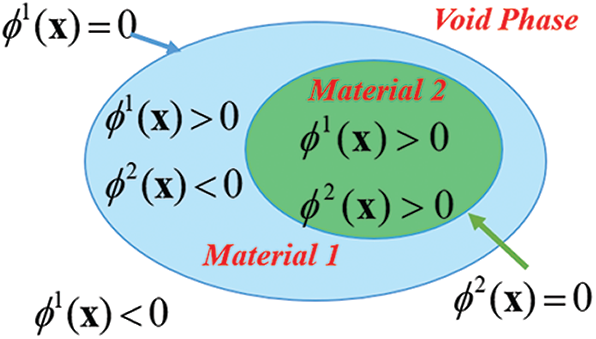
Figure 1: Multi-material system with two solid phases and one void phase via two level set functions

Then, the sensitivity of each volume fraction with respect to the design variables can be obtained from Eqs. (42a) and (42b) as, with the help of Eq. (33),

(43a)

(43b)

(43c)

(43d)

6  Numerical Results and Discussion

The linear thermoelasticity equations given in Eqs. (14) and (15) are solved using the finite element method (FEM). A fixed and rectilinear mesh is used in the homogenization-based topology optimization (e.g., [57]), and ANSYS [58] is employed as the computational tool. In addition, the level set knots are positioned at the finite element nodes for simplicity. In the examples included here, an ‘ersatz’ material model (e.g., [59]) is used to approximate material properties for those elements crossed by the moving level set boundaries, i.e., the zero level set. The volume-averaged elastic stiffness tensor Ce and coefficient of thermal expansion tensor of the eth element can be computed from Eqs. (21) and (22) through integration over the element domain as

(44)

(45)

where Ve is the volume (or area in a 2-D case) of the eth element.

When the unit cell is discretized into NE finite elements, the effective (homogenized) stiffness and thermal stress tensors given in Eqs. (10) and (11) can be written as

(46)

(47)

where

(48)

is the element stiffness matrix, is the strain-displacement matrix, denotes the element displacement under the applied strain , represents the global displacement vector associated with the element e under the mechanical loading obtainable from solving Eq. (14), and stands for the element displacement under and includes the components of the global displacement vector under thermal loading that can be computed using Eq. (15).

Further, to avoid the numerical singularity, the Heaviside function H() and the Dirac delta function involved in Eqs. (34)–(45) are approximated by the following piece-wise smooth functions [56]:

(49)

(50)

where is a real positive constant that is usually chosen as 24 times of the background cell size, and and are small positive numbers to be selected to ensure that the overall stiffness of the structure is non-singular. In this study, is taken to be 3.5 times of the average grid knot spacing, and and are selected to be 0.0001 and 0.0005, respectively.

The method of moving asymptotes (MMA) is a good optimizer in tackling multiple constraints and normally can achieve a quick convergence [52,53]. To stabilize the convergence of the optimization algorithm, the moving limit in this algorithm can be adjusted flexibly in the range of 0.05 to 0.1. In addition, the lower and upper bounds of the design variables are chosen to be and , in which c denotes the iteration cycle, is a controlling parameter ranging from 1.5 to 2, accommodating different optimization problems. The results are considered convergent when the difference between two successive iterations for the objective function is less than 0.1%.

6.1 2-D Examples

To demonstrate the procedure of topology optimization of multiphase thermoelastic metamaterials, two sets of examples are presented in this sub-section under the plane stress conditions: one is to minimize anisotropic CTE, and the other is to minimize isotropic CTE, both with a Poisson’s ratio constraint. In all of the numerical examples, the constraint of the effective bulk modulus KH is enforced to ensure the structural load-carrying capability. KH is a measurement of resistance to the volumetric strain, which, for the 2-D case, can be expressed in terms of the effective elasticity tensor components as (e.g., [48])

(51)

In all the optimizations demonstrated below, the square design domain is discretized into 60 by 60 square four-node elements, in which four Gaussian quadrature points are distributed in each direction, resulting in a total of 16 integration points in each element. For illustration purposes, material properties used in the simulations here are taken to be E1 = 1 GPa, , 1/K for solid phase 1 (in blue) and E2 = 1 GPa, , 1/K for solid phase 2 (in pink). The volume fractions for the two solid materials are specified as 25% and 10%, respectively, with a tolerance of 2%. Note that the elastic properties of the two constituent materials are chosen to be the same here to signify the effects of geometry and shape changes in the selected example problems. However, since the optimization method and the algorithm proposed here are mathematical in nature, they can be readily applied to other scenarios, where the two constituent materials have distinct (including high contrast) elastic properties, by simply changing values of the material parameters in the input file. This, of course, will lead to different optimal microstructures for the two-phase metamaterials, depending on the specified constituent properties.

Fig. 2 shows the two initial guesses employed in the topology optimization of the 2-D composites with different material distributions.

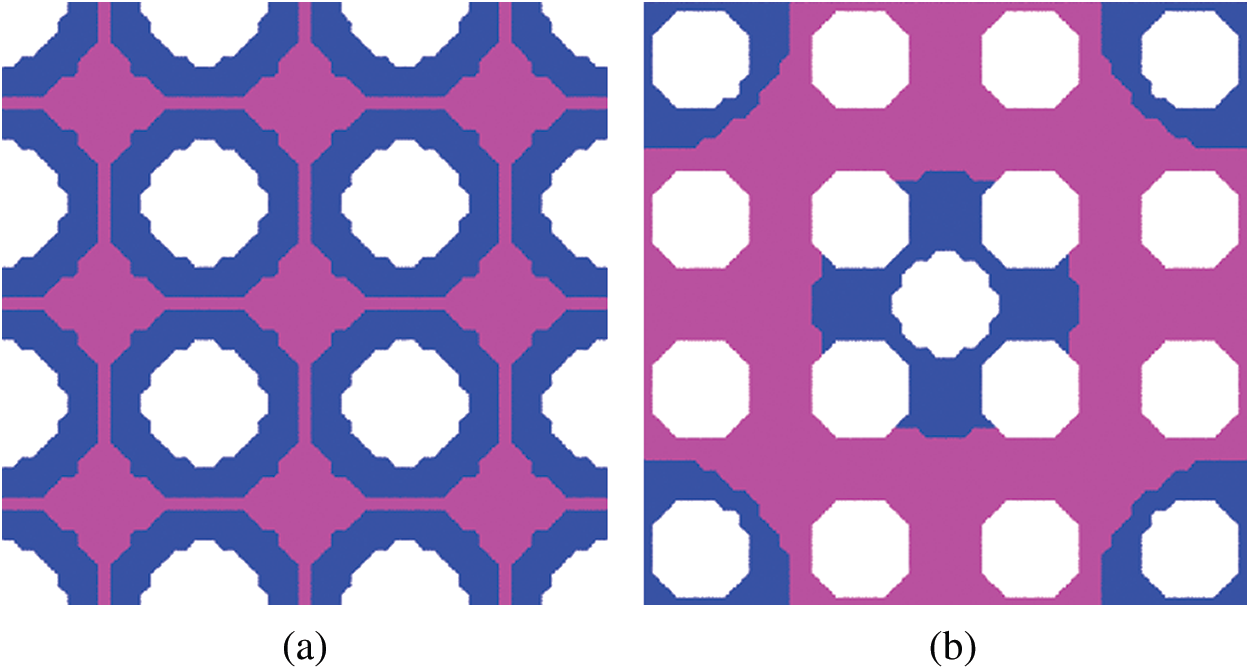
Figure 2: Initial distributions of materials in a 2-D two-phase composite: (a) case # 1, (b) case # 2

6.1.1 Minimum Anisotropic CTE with a Poisson’s Ratio Constraint

The optimization herein is to minimize the CTE in the horizontal direction , with the constraint of a positive, a zero and a negative Poisson’s ratio, respectively. The optimization starts from the two initial material distributions illustrated in Fig. 2. The constraint of 20% of the upper bound on the effective H-S bulk modulus predicted using Eq. (18b) is also enforced along with the horizontal and vertical geometrical symmetry.

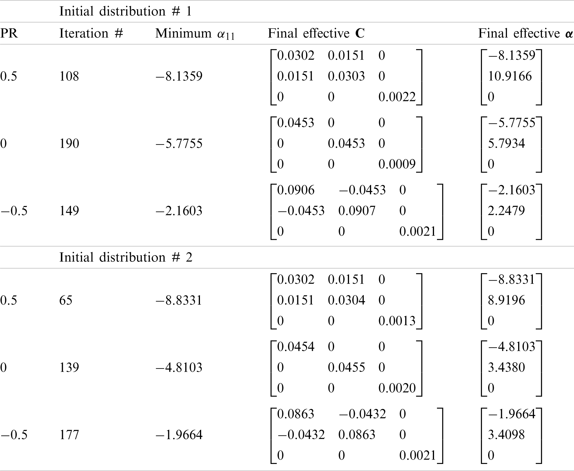
Optimal microstructures with 3-by-3 unit cells (with the single unit cell denoted by the solid green line) from the initial distribution # 1 shown in Fig. 2a are presented in Figs. 3a, 3c and 3e with the constraint of Poisson’s ratio being 0.5, 0 and −0.5, respectively. Moreover, the final optimized microstructures from the initial distribution # 2 in Fig. 2b are displayed in Figs. 4a, 4c and 4e. The plots in the right column of Figs. 3 and 4 show the iteration history curves of the objective function , Poisson’s ratio , and two volume fractions Vf1 and Vf2, respectively. The main results are summarized in Tab. 1, which contains the total number of iterations, minimum , effective elastic stiffness tensor and thermal strain tensor for all the optimization examples. It gives a side-by-side comparison of the optimization results based on the two initial distributions. It can be seen that for both of the initial distributions in Fig. 2, with the decrease of the constrained Poisson’s ratio from 0.5 to −0.5, the absolute value of the attainable minimum CTE in the x-direction decreases under the same bulk modulus constraint.

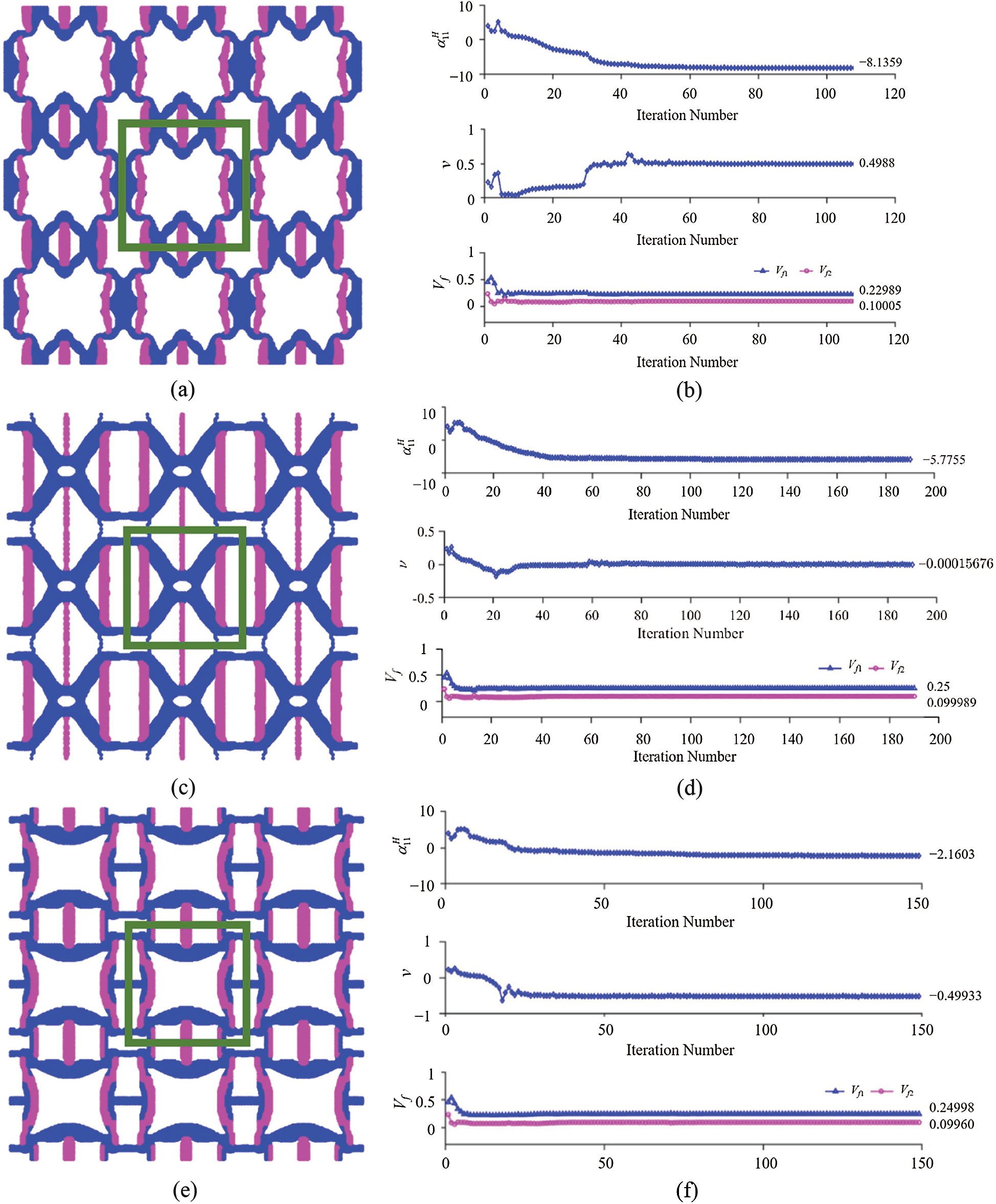
Figure 3: Minimization of with a Poisson’s ratio constraint starting from the initial distribution # 1 shown in Fig. 2a: (a) Three-by-three unit cells with PR = 0.5; (b) Iteration history with PR = 0.5 (totaling 108 iterations); (c) Three-by-three unit cells with PR = 0; (d) Iteration history with PR = 0 (totaling 190 iterations); (e) Three-by-three unit cells with PR = −0.5; (f) Iteration history with PR = −0.5 (totaling 149 iterations)

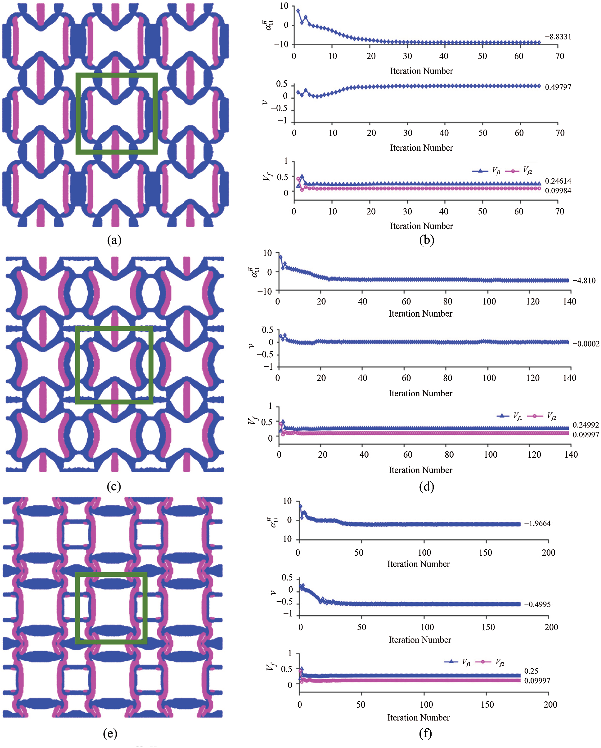
Figure 4: Minimization of with a Poisson’s ratio constraint starting from the initial distribution # 2 shown in Fig. 2b: (a) Three-by-three unit cells with PR = 0.5; (b) Iteration history with PR = 0.5 (totaling 65 iterations); (c) Three-by-three unit cells with PR = 0; (d) Iteration history with PR = 0 (totaling 139 iterations); (e) Three-by-three unit cells with PR = −0.5; (f) Iteration history with PR = −0.5 (totaling 177 iterations)

Table 1: Minimum with the Poisson’s ratio constraint based on the two initial distributions in Fig. 2

Clearly, the final optimization results based on the two initial guesses differ from each other but do not display huge differences. This is consistent with the well-known fact that final optimal designs based on the conventional level set methods tend to strongly depend on initial guesses, since the Hamilton-Jacobi PDE (see Eq. (31)) satisfies a maximum principle which prohibits the hole nucleation inside the material domain (e.g., [60]). That is, without hole nucleation mechanism in the conventional level set methods, the final optimal design will largely depend on the initial guess which dictates the maximum number of holes allowed. In order to mitigate this inherent drawback, one common and simple approach is to choose an initial guess that contains sufficiently many small holes densely distributed in the design domain, which will be allowed to merge and evolve gradually in the optimization process (e.g., [60,61]). However, this simple approach has its limitations, and more advanced techniques are needed to reduce the dependence of the level set methods on initial guesses. One of such techniques is based on the use of multiquadric radial basis functions (RBFs) to construct implicit level set functions that do not require reinitialization [60]. RBFs have been utilized in the studies on the topology optimization of 2-D mechanical metamaterials based on a parametric level set method [51] and on homogenization analyses of 3D printable interpenetrating phase composites by a meshfress method [62].

Moreover, it is observed from the optimal microstructures shown in the left column of Fig. 3 that different Poisson’s ratio constraints result in different topological features, but similarities exist due to the same initial material distribution. A comparison of the microstructures displayed in Figs. 3a, 3c and 3e shows that they all possess vertical struts with the higher CTE (in pink) that mainly control the CTE in the horizontal direction. However, the unit cell with the optimal minimum CTE under the constraint of PR = 0.5 shown in Fig. 3a has struts with the lower CTE (in blue) along the vertical direction due to the positive Poisson’s ratio constraint. For the optimal microstructure under the constraint of PR = 0 displayed in Fig. 3c, the solid material with the lower CTE (in blue) is mainly concentrated at the center of the unit cell, while most of the vertical struts comprise of the material with the higher CTE (in pink). In addition, for the optimal microstructure with the constraint of PR = −0.5 shown in Fig. 3e, an anti-chiral structure, which is known to be a main mechanism responsible for the negative Poisson’s ratio, is clearly seen. Furthermore, through comparing all the optimized results displayed in Figs. 3 and 4 based on the two initial distributions # 1 and # 2 shown in Fig. 2, it is found that the optimized microstructures with the constraint of PR = 0.5 look almost the same. However, for the other two cases with PR = 0 and PR = −0.5, the final optimal configurations resulting from the two different initial distributions display distinct topologies.

Clearly, Tab. 1 shows that the optimized 2-D composite in each case exhibits anisotropic CTEs and the cubic (for PR = 0.5 and −0.5) or isotropic (for PR = 0) elastic symmetry.

6.1.2 Minimum Isotropic CTE with a Poisson’s Ratio Constraint

The goal of this sub-section is to design microstructures with minimized isotropic CTEs and desirable Poisson’s ratios for the given horizontal and vertical symmetry. All the microstructures optimized herein possess cubic symmetry (e.g., [12]).

Figs. 5 and 6 show the optimal microstructures with 3-by-3 unit cells (with the single unit cell denoted by the solid green line) under different bulk modulus constraints, i.e., 15%, 20%, 25%, 30%, 35% and 40% of the H-R upper bound on the effective bulk modulus given by Eq. (18b), and the zero Poisson’s ratio constraint. The plots displayed in the right column of Figs. 5 and 6 show the iteration history curves of the CTE, Poisson’s ratio and two volume fractions based on the initial material distribution # 1 displayed in Fig. 2a.

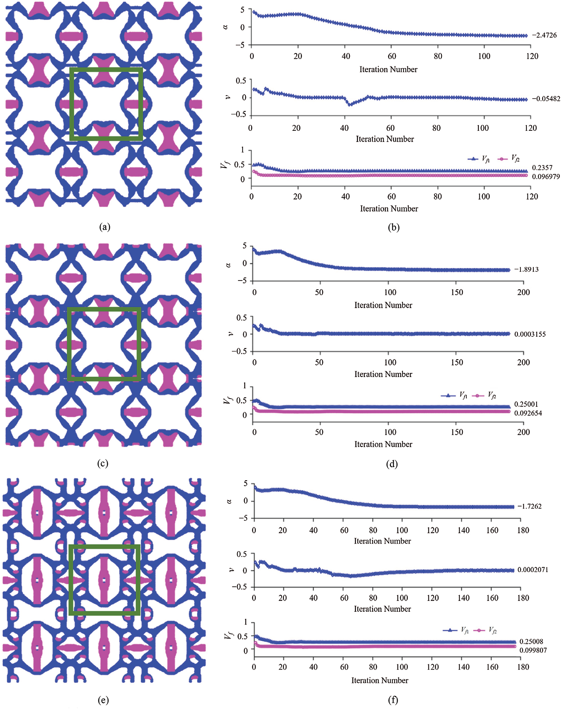
Figure 5: Minimization of isotropic CTE with the constraints of Poisson’s ratio = 0 and specified value of the bulk modulus based on the initial distribution # 1 in Fig. 2: (a), (b) Three-by-three unit cells with the bulk modulus = 15% and the iteration history (118 iterations); (c), (d) Three-by-three unit cells with the bulk modulus = 20% and the iteration history (189 iterations); (e), (f) Three-by-three unit cells with the bulk modulus = 25% and the iteration history (176 iterations)

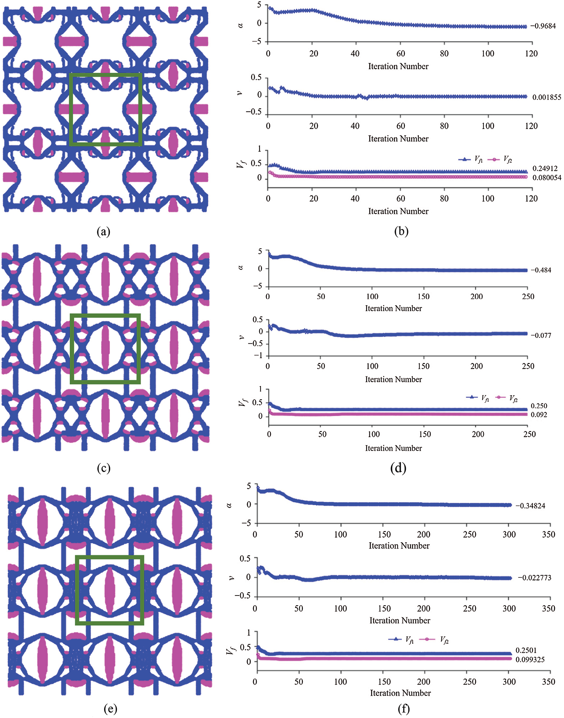
Figure 6: Minimization of isotropic CTE with the constraints of Poisson’s ratio = 0 and specified value of the bulk modulus based on the initial distribution # 1 in Fig. 2: (a), (b) Three-by-three unit cells with the bulk modulus = 30% and the iteration history (117 iterations); (c), (d) Three-by-three unit cells with the bulk modulus = 35% and the iteration history (249 iterations); (e), (f) Three-by-three unit cells with the bulk modulus = 40% and the iteration history (302 iterations)

Table 2: Minimum CTE with the constraints of different bulk modulus values and zero Poisson’s ratio from the initial distribution # 1 in Fig. 2a

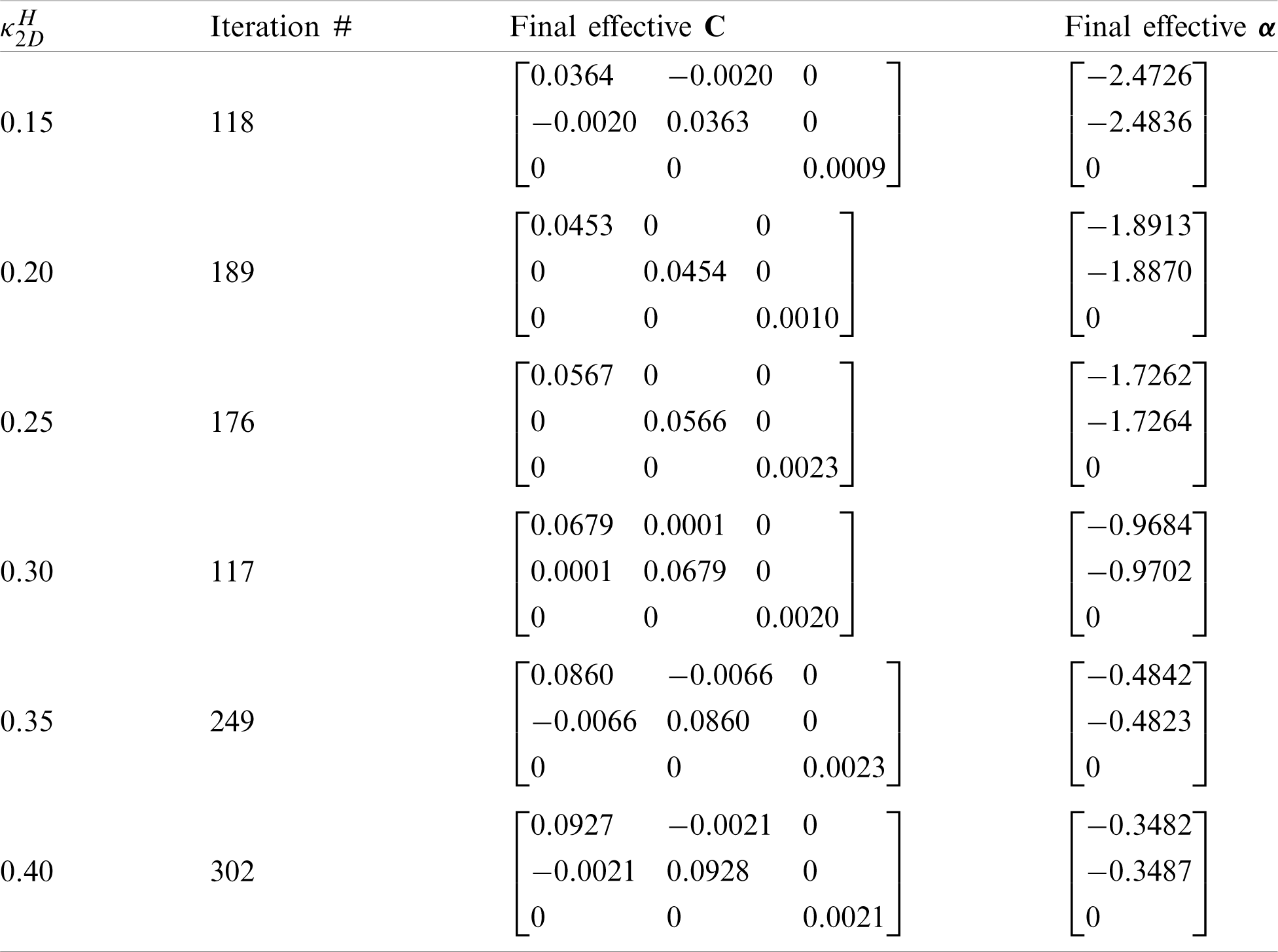
It is clearly observed from Figs. 5 and 6 that the optimized microstructures are different from each other, even though there is a detectable similarity due to the same initial distribution. Also, the microstructures with the 15%, 20% and 30% of the H-R upper bound of the effective bulk modulus displayed in Figs. 5a, 5c and 6a exhibit almost the same topological features but with different unit cell sizes. In addition, for the microstructures with the 25%, 35% and 40% of the H-R upper bound of the effective bulk modulus constraints displayed in Figs. 5e, 6c and 6e, they look slightly topologically similar but still show a significant difference. The main findings from the optimization results shown in Figs. 5 and 6 are summarized in Tab. 2, which gives a clear picture of how the effective thermoelastic properties of the optimized microstructure change with the bulk modulus constraint. It is observed that the obtained minimum isotropic CTE increases with the increase of the bulk modulus, which agrees with what is analytically predicted using Eq. (16a).

Clearly, Tab. 2 shows that the topologically optimized 2-D three-phase composite in each case exhibits isotropic CTEs and the cubic or isotropic symmetry in the elastic stiffness constants.

In addition to the topology optimization for minimizing CTE with the constraint of Poisson’s ratio = 0, simulations with the constraint of Poisson’s ratio = −0.5 are performed with the constraints of 15%, 20% and 25% of the H-R upper bounds on the effective bulk modulus given by Eq. (18b), respectively.

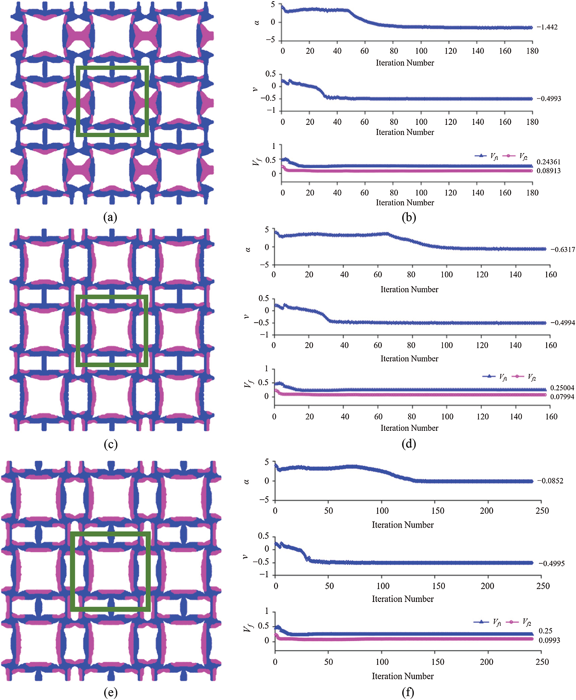
Figure 7: Minimization of isotropic CTE with the constraints of Poisson’s ratio = −0.5 and specified value of the bulk modulus based on the initial distribution # 1 displayed in Fig. 2: (a), (b) Three-by-three unit cells with the bulk modulus = 15% and the iteration history (179 iterations); (c), (d) Three-by-three unit cells with the bulk modulus = 20% and the iteration history (157 iterations); (e), (f) Three-by-three unit cells with the bulk modulus = 25% and the iteration history (241 iterations)

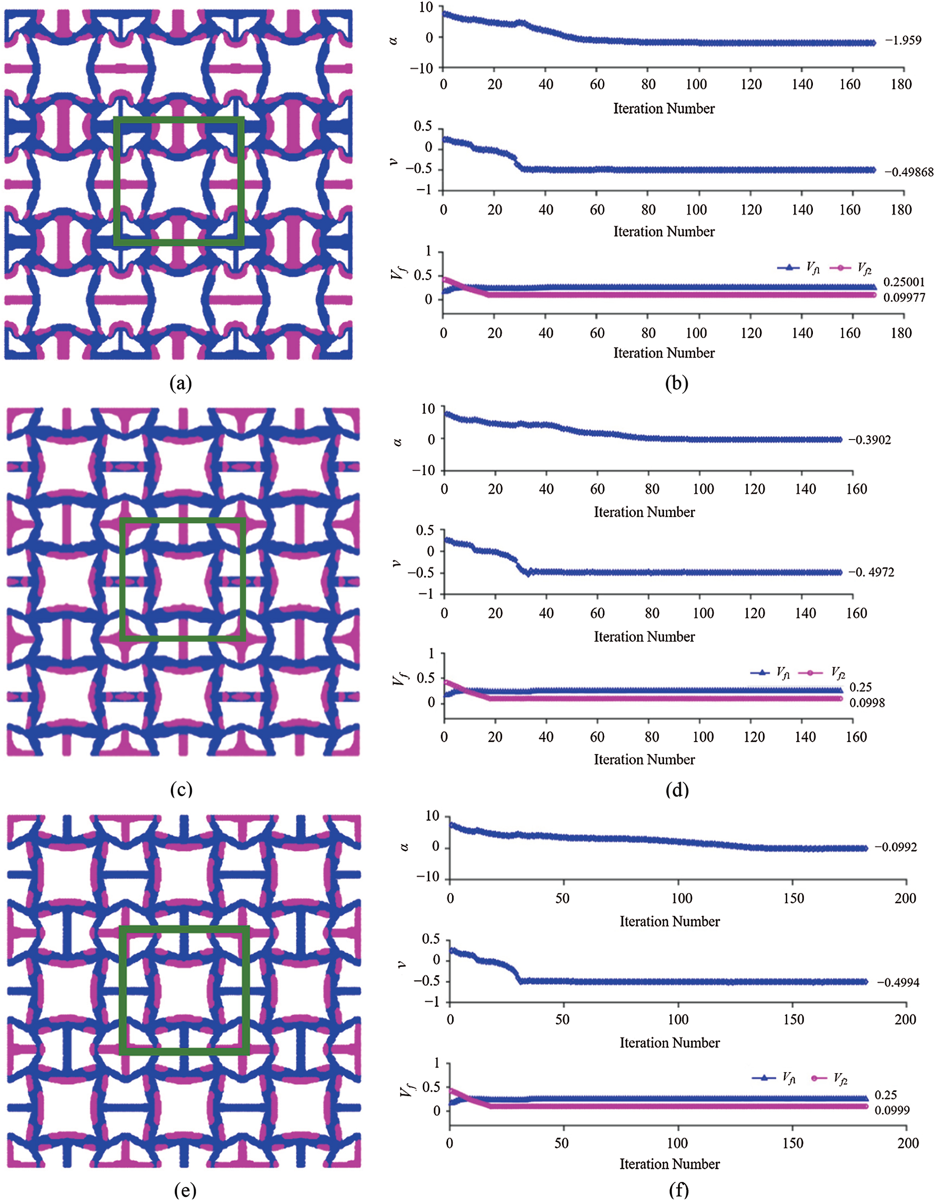
Figure 8: Minimization of isotropic CTE with the constraints of Poisson’s ratio = −0.5 and specified value of the bulk modulus based on the initial distribution # 2 shown in Fig. 2: (a), (b) Three-by-three unit cells with the bulk modulus = 15% and the iteration history (168 iterations); (c), (d) Three-by-three unit cells with the bulk modulus = 20% and the iteration history (155 iterations); (e), (f) Three-by-three unit cells with the bulk modulus = 25% and the iteration history (182 iterations)

Figs. 7 and 8 show the optimal results obtained from the two initial distributions displayed in Fig. 2. In all six numerical examples, the constraint of Poisson’s ratio = −0.5 is well maintained. Also, it is seen that the two different initial distributions lead to different microstructures with distinct minimized isotropic CTEs. For the 15% bulk modulus constraint, a minimum of −1.442 is obtained from the initial distribution # 1 and of −1.959 from the initial distribution # 2. Further, the optimal microstructures from the initial distribution # 1 contain an anti-chiral unit that is mainly responsible for the negative Poisson’s ratio, while those from the initial configuration # 2 possess a re-entrant structure, leading to a negative Poisson’s ratio of −0.5. The chirality and re-entrant structures are two well-known deformation mechanisms that can bring about negative Poisson’s ratios. Such observations are also true for the optimization with the 20% and 25% bulk modulus constraints, respectively.

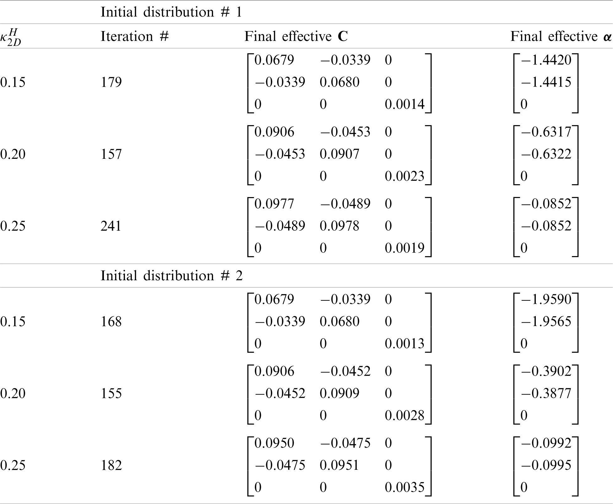
The optimization results displayed in Figs. 7 and 8 are summarized in Tab. 3, which includes the total number of iterations, the effective elastic stiffness tensor, and the coefficient of thermal expansion tensor. It is seen that the two different initial configurations lead to different optimization results, but no huge derivation exists. Moreover, the variation trend of the minimized CTE with respect to the bulk modulus constraint is the same: it increases with the increase of the bulk modulus in both cases.

Clearly, Tab. 3 shows that the topologically optimized 2-D three-phase composite in each case exhibits isotropic CTEs and the cubic symmetry in the elastic stiffness constants.

Table 3: Minimum CTE with the constraints of different bulk modulus values and Poisson’s ratio = −0.5 based on the two initial distributions displayed in Fig. 2

The effective properties of the 2-D composites with the optimal topologies shown in Figs. 5–8 are displayed as three types of markers in Fig. 9, in which the upper and lower bounds on the effective isotropic CTEs are plotted against the effective bulk modulus obtained from Eqs. (16a) and (16b). A total of 12 examples are included with the final optimal unit cells labeled from 1 to 12. As displayed at the right upper corner of the graph, all the numerical values of the effective CTE are close to the lower bound. However, through a close-up observation from Fig. 9, it is seen that the effective CTE values for the optimized microstructures with the constraint of Poisson’s ratio = 0 are much closer to the lower bound than those with the constraint of Poisson’s ratio = −0.5.

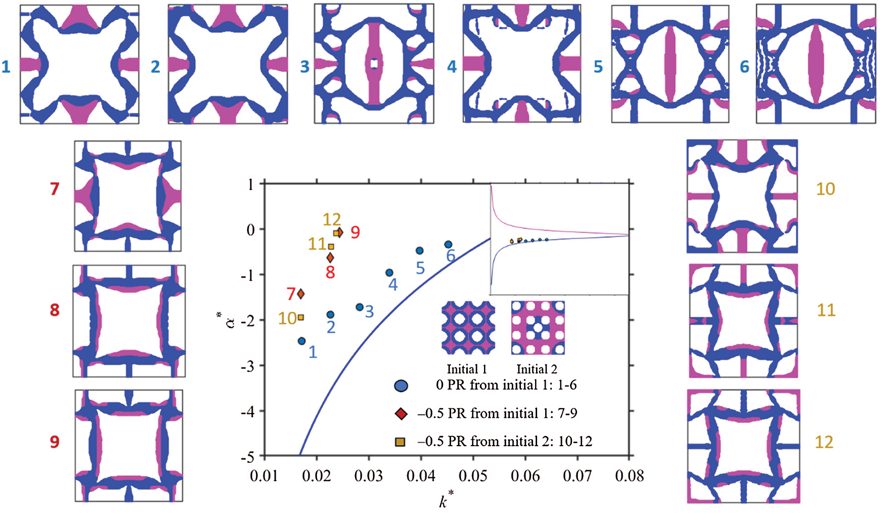
Figure 9: Effective isotropic CTE obtained from the topology optimization compared with the upper and lower bounds of the effective CTE based on Eqs. (16a) and (16b) for the 12 sample cases with the indicated optimal unit cells initially shown in Figs. 5–8

The results from Sections 6.1.1 and 6.1.2 reveal that Poisson’s ratio constraints can largely affect the extreme values of the effective CTE of a metamaterial with an optimized microstructure. The constraint of a positive Poisson’s ratio can lead to a negative CTE with a much larger magnitude than that of a negative Poisson’s ratio can. Therefore, optimal designs need to be performed to obtain metamaterials with desired negative CTEs and negative Poisson’s ratios.

6.2 3-D Examples

Similar to the 2-D multi-material and multi-objective optimizations described in Section 6.1, 3-D optimizations are performed in this sub-section. The design domain consists of 8-node brick elements with three Gaussian quadrature points distributed in each direction, resulting in a total of 27 integration points in each element. The initial 3-D design with two solid materials and one void phase is displayed in Fig. 10. For simplicity, the properties are taken to be E1 = 1 GPa, , 1/K for material 1 (in blue), and E2 = 1 GPa, , 1/K for material 2 (in pink). To demonstrate the design procedures for topology optimization of 3-D multi-phase thermoelastic metamaterials, two examples are presented here: one is to minimize anisotropic CTE, and the other is to minimize isotropic CTE. Both cases are constrained with a prescribed value of the effective Poisson’s ratio. In all the numerical examples shown below, constraints on the volume fractions are enforced along with material cubic symmetry conditions. Eqs. (46) and (47) are used to obtain the optimal effective elastic stiffness and CTE tensors for the 3-D examples presented herein.

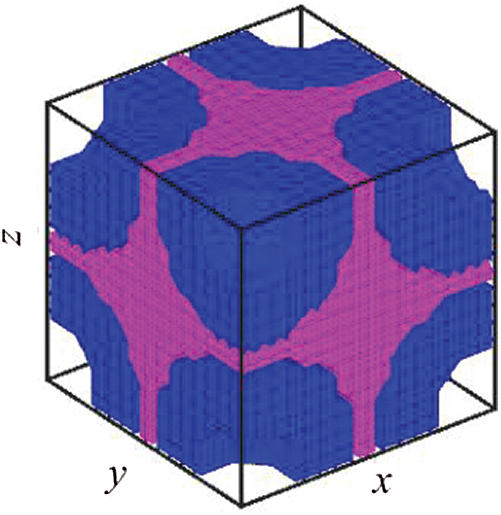
Figure 10: Initial material distribution for the 3-D case

6.2.1 Minimum Anisotropic CTE with a Poisson’s Ratio Constraint

The first case is to obtain 3-D microstructures with the minimum under the constraint of Poisson’s ratio being 0.1, 0 or −0.1. The volume fractions for the two solid materials are constrained to be 15% and 10%, respectively, with a tolerance of 2%.

Figs. 11a, 12a and 13a display the final optimal unit cells showing distributions of two solid phases. The unit cells are shown in Figs. 11b, 12b and 13b. In addition, Figs. 11c–11e, 12c–12e and 13c–13e display microstructural details from the x − y, x − z and y − z cross section views, respectively.

As shown in Figs. 11f–11h, the convergence is achieved after 116 iterations, giving a minimum of −3.4584 and a Poisson’s ratio of 0.10177 that is very close to the constrained value of 0.1 in the topology optimization problem. Furthermore, the two volume fraction constraints are well maintained: one is 0.1499, and the other is 0.099, which are almost the same as the pre-defined volume fractions of 0.15 and 0.1.

Similarly, Figs. 12f–12h show that the convergence is reached after 96 iterations, yielding a minimum of −2.7479 and a Poisson’s ratio of 0.000599, which is very close to the constrained value of zero Poisson’s ratio in the topology optimization. Moreover, the two volume fraction constraints are well maintained: one is 0.14997, and the other is 0.090172, which are almost the same as the pre-defined volume fractions of 0.15 and 0.1, with a tolerance of 2%.

For the optimization with the constraint of Poisson’s ratio = −0.1, it can be observed from Figs. 13f–13h that the convergence is achieved after 195 iterations, giving a minimum of −2.9405 and a Poisson’s ratio of −0.10213 which is quite close to the constrained value of Poisson’s ratio = −0.1 in the topology optimization. Also, the two volume fraction constraints are well maintained: one is 0.14795, and the other is 0.080033, which are very close to the pre-defined volume fractions of 0.15 and 0.1, with a tolerance of 2%.

Note that the magnitude of −3.4584 obtained with the constraint of Poisson’s ratio = 0.1 is larger than that of under the constraint of Poisson’s ratio = 0, which is smaller than the magnitude of obtained with Poisson’s ratio = −0.1. This indicates that the Poisson’s ratio and CTE are not directly related and can therefore be independently varied without affecting each another, which agrees with what was found in [19].

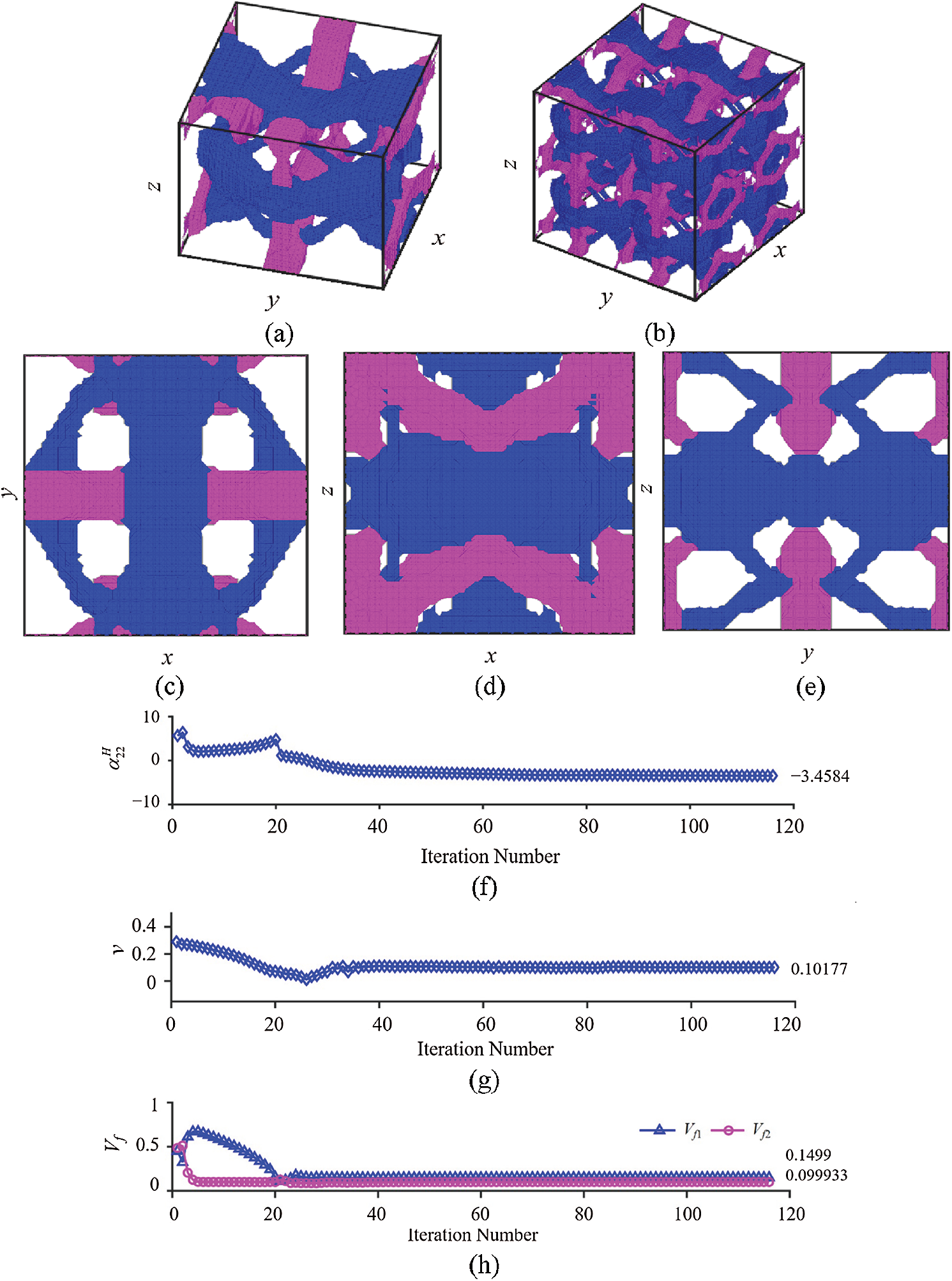
Figure 11: Minimization of under the constraint of Poisson’s ratio = 0.1: (a) Optimal unit cell; (b) Periodic microstructures with unit cells; (c) Unit cell in the x − y cross section view; (d) Unit cell in the x − z cross section view; (e) Unit cell in the y − z cross section view; (f) Iteration history of CTE in the y-direction; (g) Iteration history of Poisson’s ratio; (h) Iteration history of two volume fraction constraints (total 116 iterations to achieve convergence)

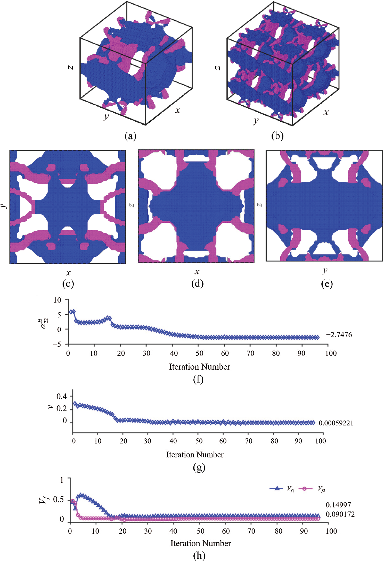
Figure 12: Minimization of under the constraint of Poisson’s ratio = 0: (a) Optimal unit cell; (b) Periodic microstructures with unit cells; (c) Unit cell in the x − y cross section view; (d) Unit cell in the x − z cross section view; (e) Unit cell in the y − z cross section view; (f) Iteration history of CTE in the y-direction; (g) Iteration history of Poisson’s ratio; (h) Iteration history of two volume fraction constraints (total 96 iterations to achieve convergence)

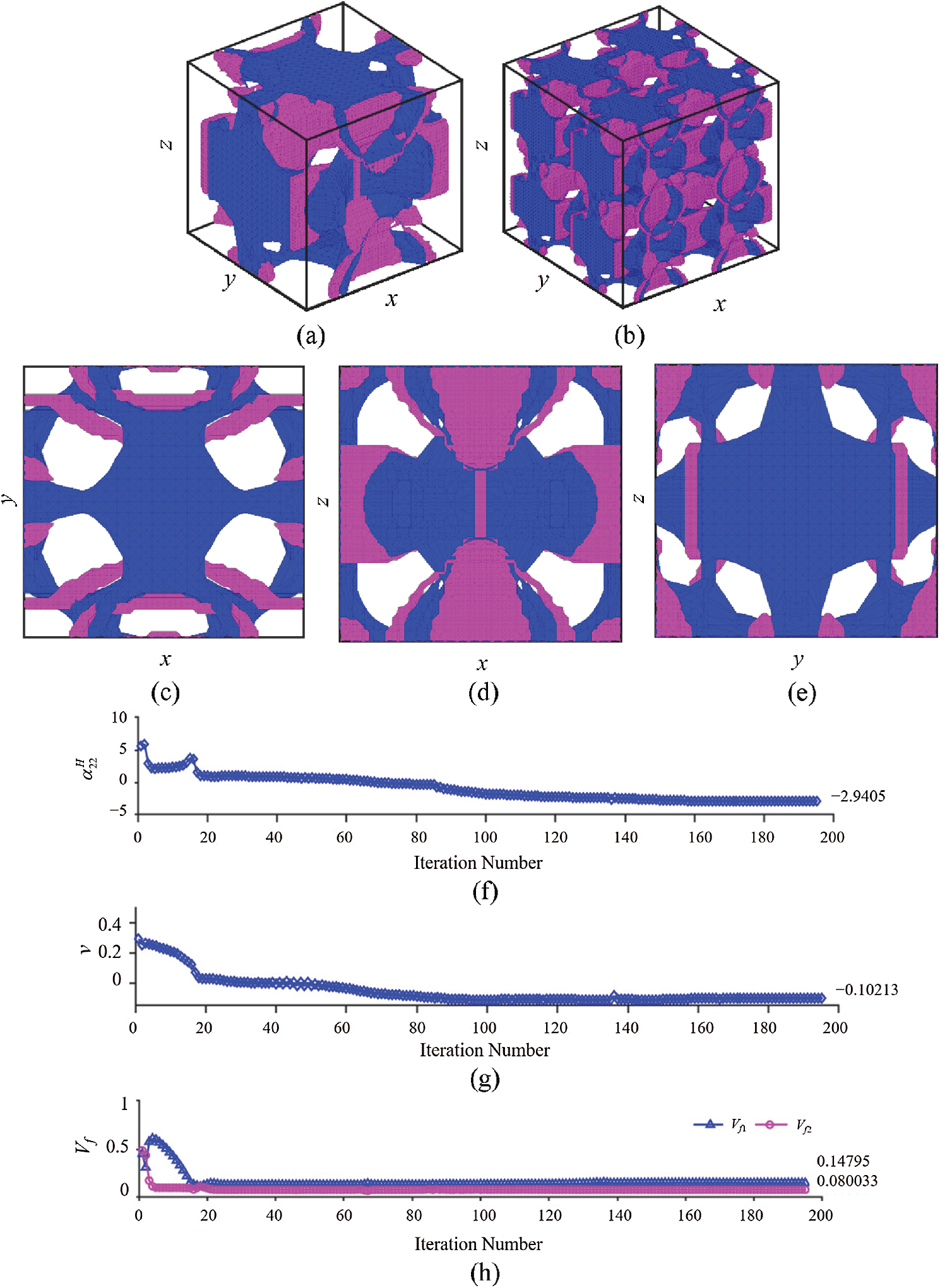
Figure 13: Minimization of under the constraint of Poisson’s ratio = −0.1: (a) Optimal unit cell; (b) Periodic microstructures with unit cells; (c) Unit cell in the x − y cross section view; (d) Unit cell in the x − z cross section view; (e) Unit cell in the y − z cross section view; (f) Iteration history of CTE in the y-direction; (g) Iteration history of Poisson’s ratio; (h) Iteration history of two volume fraction constraints (total 195 iterations to achieve convergence)

Figs. 11–13 show 3-D optimal microstructures with complex topologies achieved through the optimization evolution process originated from the initial design illustrated in Fig. 10. This indicates that the approach employed in the current study is capable of merging and creating holes without implementing topological derivatives [63] or other techniques. Also, it is seen that the present approach can integrate shape and topology optimizations, in which the first few iterations are used to quickly achieve the optimal topology and the rest of iterations before the final convergence are mainly serving to complete the shape optimization.

The effective elastic stiffness and CTE tensors for the three optimal microstructures with different Poisson’s ratio constraints shown in Figs. 11–13 are, respectively, obtained as

(52)

(53)

(54)

Clearly, Eqs. (52)–(54) show that the topologically optimized 3-D three-phase composite in each case exhibits anisotropic CTEs and elastic stiffness constants that satisfy the cubic symmetry.

It should be pointed out that the optimal geometrical boundaries shown in Figs. 11–13 appear to have serrated shapes that are not sufficiently smooth. The reason for this is that the total number of elements used here is 13824 in a mesh, which is not fine enough to produce smooth boundaries but remains a limitation of the current study for the 3-D three-phase metamaterials. In addition, it can be observed that the same initial structures could lead to distinctive designs if they have been given different constraints even with the same objective function. Alternatively, the different initial distributions lead to different final optimal microstructures owing to the highly non-convex problems with multiple local regions existing in the current gradient-based optimization enabled by the PLSM (e.g., [60]).

From the unit cells displayed in Figs. 11–13, it is not easy to tell underlying mechanisms that may lead to the desired negative CTE and Poisson’s ratio, unlike that for the 2-D cases described in Section 6.1. This is a feature inherent in topology optimization that could result in designs unattainable through conventional thinking.

6.2.2 Minimum Isotropic CTE with a Poisson’s Ratio Constraint

The goal here is to obtain the minimum isotropic CTE under the constraints of Poisson’s ratio being 0 and the volume fractions of the two solid materials at 15% and 6%, respectively, with a tolerance of 2%.

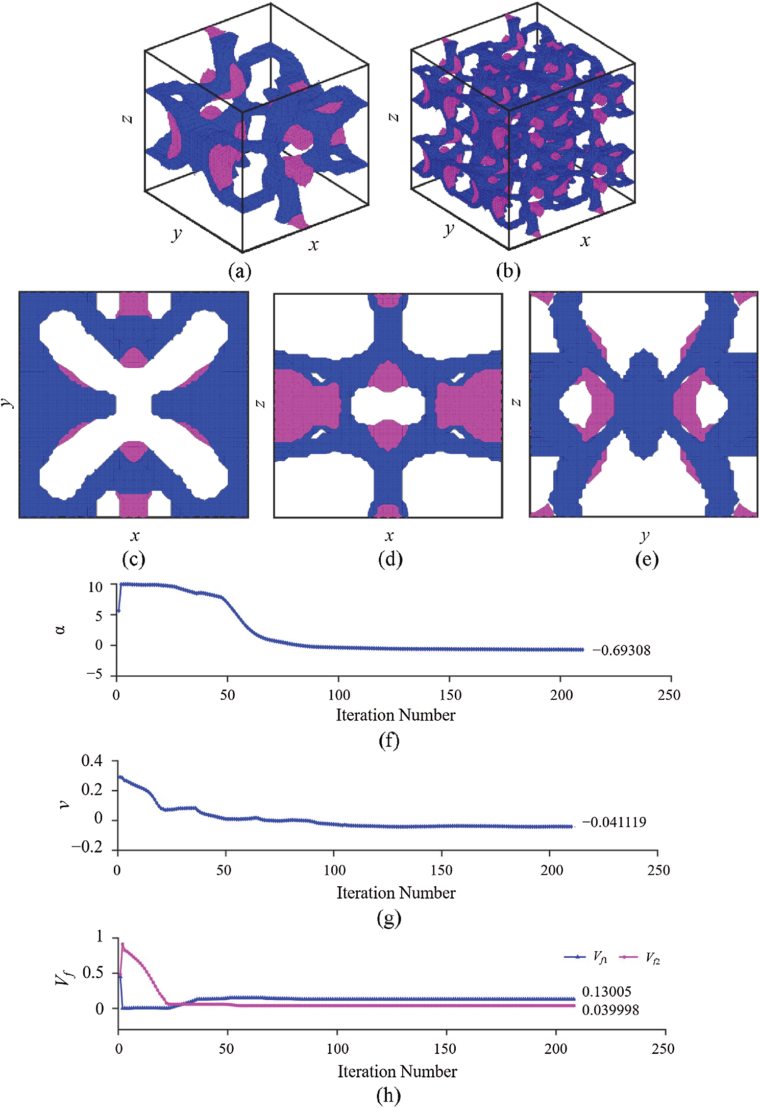
Figure 14: Minimization of isotropic CTE under the zero Poisson’s ratio constraint: (a) Optimal unit cell; (b) Periodic microstructures with unit cells; (c) Unit cell in the x − y cross section view; (d) Unit cell in the x − z cross section view; (e) Unit cell in the y − z cross section view; (f) Iteration history of CTE; (g) Iteration history of Poisson’s ratio; (h) Iteration history of the two volume fraction constraints (totalling 210 iterations to achieve convergence)

Fig. 14a displays the optimal unit cell, and Fig. 14b shows periodic unit cells. It can be seen that very clear and distinct material interfaces are formed between the two solid phases that can be reconstructed with ease from the mesh generated in topology optimization. In addition, Figs. 14c–14e provide the 2-D cross-sectional views from three perspectives that further demonstrate fine geometrical features obtained from topology optimization. Furthermore, Figs. 14f–14h give the convergence plots for the effective CTE, Poisson’s ratio, and two volume fraction constraints, in which 210 iterations are performed to achieve the final results with the CTE being −0.69308, Poisson’s ratio −0.0411 and two volume fractions 0.13005 and 0.04, respectively. For the solid material with the higher CTE displayed in pink, the volume fraction first jumps to about 90% and then gradually drops down to satisfy the volume fraction constraint in the topology optimization. On the other hand, for the solid phase with the lower CTE (marked in blue), it drops from the initial volume fraction of 48% down to near zero and then increases to achieve the required volume fraction. Moreover, the optimization approaches adopted here work pretty well concerning the hole nucleation and merging.

The effective elastic stiffness and CTE tensors for the optimal microstructure generated in this case are obtained as

(55)

From Eq. (55), it is seen that the topologically optimized 3-D three-phase composite in this case shows an isotropic CTE and elastic stiffness constants satisfying the cubic symmetry.

Finally, it should be mentioned that fabricating the 3-D multi-phase metamaterial samples discussed here by using traditional subtractive manufacturing techniques is very challenging. However, additive manufacturing methods can be employed to print these optimally designed composite structures (e.g., [64]). Topologically optimized 2-D multiphase polymeric metamaterials with a tunable CTE have been produced by additive manufacturing through an Objet Connex 500 3D printer (e.g., [25]).

7  Conclusion

A parametric level set-based topology optimization method is used to design 2-D and 3-D multiphase thermoelastic metamaterials with minimized anisotropic and isotropic CTEs and prescribed values of Poisson’s ratio under the constraints of specified effective bulk modulus, volume fractions and material symmetry. The effective properties of the multiphase metamaterials are predicted using an asymptotic homogenization method. The -constraint multi-objective optimization method is utilized in the formulation, and the method of moving asymptotes is employed to solve the optimization problems.

In each design example considered, two solid materials and one void phase are included. It is found that optimal 2-D and 3-D microstructures can be generated by applying the newly proposed approach. Novel structures are obtained through the current topology optimization approach, which are difficult to achieve using conventional (heuristic) methods. In addition, the new approach can lead to topologically optimized metamaterials with a positive, negative or zero Poisson’s ratio and a positive, negative or zero CTE.

Acknowledgement: The authors gratefully thank Prof. Krister Svanberg for providing his MMA codes to us. We also would like to thank two anonymous reviewers for their encouragement and helpful comments on an earlier version of the paper.

Funding Statement: The authors received no specific funding for this study.

Conflicts of Interest: The authors declare that they have no conflicts of interest to report regarding the present study.

References

 1.  Ha, C. S., Hestekin, E., Li, J. H., Plesha, M. E., Lakes, R. S. (2015). Controllable thermal expansion of large magnitude in chiral negative Poisson’s ratio lattices. Physica Status Solidi (B), 252(7), 1431–1434. DOI 10.1002/pssb.201552158. [Google Scholar] [CrossRef]

 2.  Xu, H., Pasini, D. (2016). Structurally efficient three-dimensional metamaterials with controllable thermal expansion. Scientific Reports, 6(1), 34924. DOI 10.1038/srep34924. [Google Scholar] [CrossRef]

 3.  Zadpoor, A. A. (2016). Mechanical meta-materials. Materials Horizons, 3(5), 371–381. DOI 10.1039/C6MH00065G. [Google Scholar] [CrossRef]

 4.  Hewage, T. A., Alderson, K. L., Alderson, A., Scarpa, F. (2016). Double-negative mechanical metamaterials displaying simultaneous negative stiffness and negative Poisson’s ratio properties. Advanced Materials, 28(46), 10323–10332. DOI 10.1002/adma.201603959. [Google Scholar] [CrossRef]

 5.  Chen, Y. Y., Li, T. T., Scarpa, F., Wang, L. F. (2017). Lattice metamaterials with mechanically tunable Poisson’s ratio for vibration control. Physical Review Applied, 7(2), 24012. DOI 10.1103/PhysRevApplied.7.024012. [Google Scholar] [CrossRef]

 6.  Ren, X., Das, R., Tran, P., Ngo, T. D., Xie, Y. M. (2018). Auxetic metamaterials and structures: A review. Smart Materials and Structures, 27(2), 023001. DOI 10.1088/1361-665X/aaa61c. [Google Scholar] [CrossRef]

 7.  Wang, Y. J., Liao, Z. Y., Shi, S. Y., Wang, Z. P., Poh, L. H. (2020). Data-driven structural design optimization for petal-shaped auxetics using isogeometric analysis. Computer Modeling in Engineering & Sciences, 122(2), 433–458. DOI 10.32604/cmes.2020.08680. [Google Scholar] [CrossRef]

 8.  Lakes, R. S. (2007). Cellular solids with tunable positive or negative thermal expansion of unbounded magnitude. Applied Physics Letters, 90(22), 221905. DOI 10.1063/1.2743951. [Google Scholar] [CrossRef]

 9.  Steeves, C. A., Lucato, S. L. D. S., He, M., Antinucci, E., Hutchinson, J. W. et al. (2007). Concepts for structurally robust materials that combine low thermal expansion with high stiffness. Journal of the Mechanics and Physics of Solids, 55(9), 1803–1822. DOI 10.1016/j.jmps.2007.02.009. [Google Scholar] [CrossRef]

10. Li, T. T., Hu, X. Y., Chen, Y. Y., Wang, L. F. (2017). Harnessing out-of-plane deformation to design 3D architected lattice metamaterials with tunable Poisson’s ratio. Scientific Reports, 7(1), 8949. DOI 10.1038/s41598-017-09218-w. [Google Scholar] [CrossRef]

11. Ai, L., Gao, X. L. (2017). Metamaterials with negative Poisson’s ratio and non-positive thermal expansion. Composite Structures, 162, 70–84. DOI 10.1016/j.compstruct.2016.11.056. [Google Scholar] [CrossRef]

12. Ai, L., Gao, X. L. (2017). Micromechanical modeling of 3-D printable interpenetrating phase composites with tailorable effective elastic properties including negative Poisson’s ratio. Journal of Micromechanics and Molecular Physics, 2(4), 1750015. DOI 10.1142/S2424913017500151. [Google Scholar] [CrossRef]

13. Ai, L., Gao, X. L. (2018). Three-dimensional metamaterials with a negative Poisson’s ratio and a non-positive coefficient of thermal expansion. International Journal of Mechanical Sciences, 135(7), 101–113. DOI 10.1016/j.ijmecsci.2017.10.042. [Google Scholar] [CrossRef]

14. Ai, L., Gao, X.-L. (2018). An analytical model for star-shaped re-entrant lattice structures with the orthotropic symmetry and negative Poisson’s ratios. International Journal of Mechanical Sciences, 145(1), 158–170. DOI 10.1016/j.ijmecsci.2018.06.027. [Google Scholar] [CrossRef]

15. Sigmund, O., Maute, K. (2013). Topology optimization approaches: A comparative review. Structural and Multidisciplinary Optimization, 48(6), 1031–1055. DOI 10.1007/s00158-013-0978-6. [Google Scholar] [CrossRef]

16. Wang, Y., Lu, E., Zhao, J., Guo, J. (2015). Meshfree method for the topological design of microstructural composites. Computer Modeling in Engineering & Sciences, 109, 35–53. DOI 10.3970/cmes.2015.109.035. [Google Scholar] [CrossRef]

17. Osanov, M., Guest, J. K. (2016). Topology optimization for architected materials design. Annual Review of Materials Research, 46(1), 211–233. DOI 10.1146/annurev-matsci-070115-031826. [Google Scholar] [CrossRef]

18. Wang, Y. J., Wang, Z. P., Xia, Z. H., Poh, L. H. (2018). Structural design optimization using isogeometric analysis: A comprehensive review. Computer Modeling in Engineering & Sciences, 117(3), 455–507. DOI 10.31614/cmes.2018.04603. [Google Scholar] [CrossRef]

19. Sigmund, O., Torquato, S. (1996). Composites with extremal expansion coefficients. Applied Physics Letters, 69(21), 3203–3205. DOI 10.1063/1.117961. [Google Scholar] [CrossRef]

20. Sigmund, O., Torquato, S. (1997). Design of materials with extreme thermal expansion using a three-phase topology optimization method. Journal of the Mechanics and Physics of Solids, 45(6), 1037–1067. DOI 10.1016/S0022-5096(96)00114-7. [Google Scholar] [CrossRef]

21. Schwerdtfeger, J., Wein, F., Leugering, G., Singer, R. F., Körner, C. et al. (2011). Design of auxetic structures via mathematical optimization. Advanced Materials, 23(22–23), 2650–2654. DOI 10.1002/adma.201004090. [Google Scholar] [CrossRef]

22. Andreassen, E., Lazarov, B. S., Sigmund, O. (2014). Design of manufacturable 3D extremal elastic microstructure. Mechanics of Materials, 69(1), 1–10. DOI 10.1016/j.mechmat.2013.09.018. [Google Scholar] [CrossRef]

23. Wang, Y., Luo, Z., Zhang, N., Wu, T. (2016). Topological design for mechanical metamaterials using a multiphase level set method. Structural and Multidisciplinary Optimization, 54(4), 937–952. DOI 10.1007/s00158-016-1458-6. [Google Scholar] [CrossRef]

24. Vogiatzis, P., Chen, S., Wang, X., Li, T., Wang, L. (2017). Topology optimization of multi-material negative Poisson’s ratio metamaterials using a reconciled level set method. Computer-Aided Design, 83, 15–32. DOI 10.1016/j.cad.2016.09.009. [Google Scholar] [CrossRef]

25. Takezawa, A., Kobashi, M. (2017). Design methodology for porous composites with tunable thermal expansion produced by multi-material topology optimization and additive manufacturing. Composites Part B: Engineering, 131(4), 21–29. DOI 10.1016/j.compositesb.2017.07.054. [Google Scholar] [CrossRef]

26. Wang, Y., Gao, J., Luo, Z., Brown, T., Zhang, N. (2017). Level-set topology optimization for multimaterial and multifunctional mechanical metamaterials. Engineering Optimization, 49(1), 22–42. DOI 10.1080/0305215X.2016.1164853. [Google Scholar] [CrossRef]

27. Ye, M. L., Gao, L., Li, H. (2020). A design framework for gradually stiffer mechanical metamaterial induced by negative Poisson’s ratio property. Materials & Design, 192(4), 108751. DOI 10.1016/j.matdes.2020.108751. [Google Scholar] [CrossRef]

28. Li, H., Li, H., Xiao, M., Zhang, Y., Fu, J. et al. (2020). Robust topology optimization of thermoelastic metamaterials considering hybrid uncertainties of material property. Composite Structures, 248(2), 112477. DOI 10.1016/j.compstruct.2020.112477. [Google Scholar] [CrossRef]

29. Hassani, B., Hinton, E. (1998). A review of homogenization and topology optimization I–homogenization theory for media with periodic structure. Computers and Structures, 69(6), 707–717. DOI http://dx.doi.org/10.1016/S0045-7949(98)00131-X. [Google Scholar]

30. Li, S., Wang, G. (2008). Introduction to micromechanics and nanomechanics. Singapore: World Scientific. [Google Scholar]

31. Kalamkarov, A. L., Andrianov, I. V., Danishevsâ, V. V. (2009). Asymptotic homogenization of composite materials and structures. Applied Mechanics Reviews, 62(3), 30802. DOI 10.1115/1.3090830. [Google Scholar] [CrossRef]

32. Nasution, M. R. E., Watanabe, N., Kondo, A., Yudhanto, A. (2014). Thermomechanical properties and stress analysis of 3-D textile composites by asymptotic expansion homogenization method. Composites Part B: Engineering, 60(4), 378–391. DOI 10.1016/j.compositesb.2013.12.038. [Google Scholar] [CrossRef]

33. Sigmund, O. (1995). Tailoring materials with prescribed elastic properties. Mechanics of Materials, 20(4), 351–368. DOI 10.1016/0167-6636(94)00069-7. [Google Scholar] [CrossRef]

34. Turner, P. S. (1946). Thermal expansion stresses in reinforced plastics. Journal of Research of the National Bureau of Standards, 37(4), 239–250. DOI 10.6028/jres.037.015. [Google Scholar] [CrossRef]

35. Schapery, R. A. (1968). Thermal expansion coefficients of composite materials based on energy principles. Journal of Composite Materials, 2(3), 380–404. DOI 10.1177/002199836800200308. [Google Scholar] [CrossRef]

36. Rosen, B. W., Hashin, Z. (1970). Effective thermal expansion coefficients and specific heat of composite materials. International Journal of Engineering, 8(2), 157–173. DOI 10.1016/0020-7225(70)90066-2. [Google Scholar] [CrossRef]

37. Gibiansky, L. V., Torquato, S. (1997). Thermal expansion of isotropic multiphase composites and polycrystals. Journal of the Mechanics and Physics of Solids, 45(7), 1223–1252. DOI 10.1016/S0022-5096(96)00129-9. [Google Scholar] [CrossRef]

38. Hashin, Z., Shtrikman, S. (1963). A variational approach to the theory of the elastic behaviour of multiphase materials. Journal of the Mechanics and Physics of Solids, 11(2), 127–140. DOI 10.1016/0022-5096(63)90060-7. [Google Scholar] [CrossRef]

39. Gibiansky, L. V., Sigmund, O. (2000). Multiphase composites with extremal bulk modulus. Journal of the Mechanics and Physics of Solids, 48(3), 461–498. DOI 10.1016/S0022-5096(99)00043-5. [Google Scholar] [CrossRef]

40. Jasiuk, I., Chen, J., Thorpe, M. F. (1994). Elastic moduli of two dimensional materials with polygonal and elliptical holes. Applied Mechanics Reviews, 47(1S), 18–28. DOI 10.1115/1.3122813. [Google Scholar] [CrossRef]

41. Luo, Z., Tong, L., Wang, M. Y., Wang, S. (2007). Shape and topology optimization of compliant mechanisms using a parameterization level set method. Journal of Computational Physics, 227(1), 680–705. DOI 10.1016/j.jcp.2007.08.011. [Google Scholar] [CrossRef]

42. Luo, Z., Tong, L. (2008). A level set method for shape and topology optimization of large-displacement compliant mechanisms. International Journal for Numerical Methods in Engineering, 76(6), 862–892. DOI 10.1002/nme.2352. [Google Scholar] [CrossRef]

43. van Dijk, N. P., Maute, K., Langelaar, M., van Keulen, F. (2013). Level-set methods for structural topology optimization: A review. Structural and Multidisciplinary Optimization, 48(3), 437–472. DOI 10.1007/s00158-013-0912-y. [Google Scholar] [CrossRef]

44. Wang, Y. Q., Luo, Z., Kang, Z., Zhang, N. (2015). A multi-material level set-based topology and shape optimization method. Computer Methods in Applied Mechanics and Engineering, 283(21), 1570–1586. DOI 10.1016/j.cma.2014.11.002. [Google Scholar] [CrossRef]

45. Wang, M. Y., Wang, X. (2004). Color level sets: A multi-phase method for structural topology optimization with multiple materials. Computer Methods in Applied Mechanics and Engineering, 193(6–8), 469–496. DOI 10.1016/j.cma.2003.10.008. [Google Scholar] [CrossRef]

46. Luo, Z., Tong, L., Luo, J., Wei, P., Wang, M. Y. (2009). Design of piezoelectric actuators using a multiphase level set method of piecewise constants. Journal of Computational Physics, 228(7), 2643–2659. DOI 10.1016/j.jcp.2008.12.019. [Google Scholar] [CrossRef]

47. Guest, J. K., Prévost, J. H. (2006). Optimizing multifunctional materials: Design of microstructures for maximized stiffness and fluid permeability. International Journal of Solids and Structures, 43(22–23), 7028–7047. DOI 10.1016/j.ijsolstr.2006.03.001. [Google Scholar] [CrossRef]

48. de Kruijf, N., Zhou, S., Li, Q., Mai, Y. W. (2007). Topological design of structures and composite materials with multiobjectives. International Journal of Solids and Structures, 44(22–23), 7092–7109. DOI 10.1016/j.ijsolstr.2007.03.028. [Google Scholar] [CrossRef]

49. Mavrotas, G. (2009). Effective implementation of the -constraint method in multi-objective mathematical programming problems. Applied Mathematics and Computation, 213(2), 455–465. DOI 10.1016/j.amc.2009.03.037. [Google Scholar] [CrossRef]

50. Kunakote, T., Bureerat, S. (2011). Multi-objective topology optimization using evolutionary algorithms. Engineering Optimization, 43(5), 541–557. DOI 10.1080/0305215X.2010.502935. [Google Scholar] [CrossRef]

51. Ai, L., Gao, X. L. (2019). Topology optimization of 2-D mechanical metamaterials using a parametric level set method combined with a meshfree algorithm. Composite Structures, 229(5), 111318. DOI 10.1016/j.compstruct.2019.111318. [Google Scholar] [CrossRef]

52. Svanberg, K. (1987). The method of moving asymptotes—A new method for structural optimization. International Journal for Numerical Methods in Engineering, 24(2), 359–373. DOI 10.1002/nme.1620240207. [Google Scholar] [CrossRef]

53. Svanberg, K. (2002). A class of globally convergent optimization methods based on conservative convex separable approximations. SIAM Journal on Optimization, 12(2), 555–573. DOI 10.1137/S1052623499362822. [Google Scholar] [CrossRef]

54. Deng, J., Yan, J., Cheng, G. (2013). Multi-objective concurrent topology optimization of thermoelastic structures composed of homogeneous porous material. Structural and Multidisciplinary Optimization, 47(4), 583–597. DOI 10.1007/s00158-012-0849-6. [Google Scholar] [CrossRef]

55. Bower, A. F. (2009). Applied mechanics of solids. Boca Raton, FL: CRC Press. [Google Scholar]

56. Wang, M. Y., Wang, X., Guo, D. (2003). A level set method for structural topology optimization. Computer Methods in Applied Mechanics and Engineering, 192(1–2), 227–246. DOI 10.1016/S0045-7825(02)00559-5. [Google Scholar] [CrossRef]

57. Andreassen, E., Andreasen, C. S. (2014). How to determine composite material properties using numerical homogenization. Computational Materials Science, 83, 488–495. DOI 10.1016/j.commatsci.2013.09.006. [Google Scholar] [CrossRef]

58. ANSYS (2017). ANSYS mechanical APDL structural analysis guide. Canonsburg, PA: ANSYS, Inc. [Google Scholar]

59. Allaire, G., Jouve, F., Toader, A.-M. (2004). Structural optimization using sensitivity analysis and a level-set method. Journal of Computational Physics, 194(1), 363–393. DOI 10.1016/j.jcp.2003.09.032. [Google Scholar] [CrossRef]

60. Wang, S. Y., Lim, K. M., Khoo, B. C., Wang, M. Y. (2007). An extended level set method for shape and topology optimization. Journal of Computational Physics, 221(1), 395–421. DOI 10.1016/j.jcp.2006.06.029. [Google Scholar] [CrossRef]

61. Tsai, R., Osher, S. (2003). Level set methods and their applications in image science. Communications in Mathematical Sciences, 1(4), 623–656. [Google Scholar]

62. Ai, L., Gao, X. L. (2018). Evaluation of effective elastic properties of 3-D printable interpenetrating phase composites using the meshfree radial point interpolation method. Mechanics of Advanced Materials and Structures, 25(15–16), 1241–1251. DOI 10.1080/15376494.2016.1143990. [Google Scholar] [CrossRef]

63. Burger, M., Hackl, B., Ring, W. (2004). Incorporating topological derivatives into level set methods. Journal of Computational Physics, 194(1), 344–362. DOI 10.1016/j.jcp.2003.09.033. [Google Scholar] [CrossRef]

64. Rafiee, M., Farahani, R. D., Therriault, D. (2020). Multi-material 3D and 4D printing: A survey. Advanced Science, 7(12), 1902307. DOI 10.1002/advs.201902307. [Google Scholar] [CrossRef]

This work is licensed under a Creative Commons Attribution 4.0 International License, which permits unrestricted use, distribution, and reproduction in any medium, provided the original work is properly cited.