Engineering & Sciences
| Computer Modeling in Engineering & Sciences |
DOI: 10.32604/cmes.2021.014469
ARTICLE
Hybrid Effects of Thermal and Concentration Convection on Peristaltic Flow of Fourth Grade Nanofluids in an Inclined Tapered Channel: Applications of Double-Diffusivity
MCS, National University of Sciences and Technology, Islamabad, Pakistan
*Corresponding Author: Safia Akram. Email: drsafiaakram@gmail.com; drsafiaakram@mcs.edu.pk
Received: 29 September 2020; Accepted: 04 January 2021
Abstract: This article brings into focus the hybrid effects of thermal and concentration convection on peristaltic pumping of fourth grade nanofluids in an inclined tapered channel. First, the brief mathematical modelling of the fourth grade nanofluids is provided along with thermal and concentration convection. The Lubrication method is used to simplify the partial differential equations which are tremendously nonlinear. Further, analytical technique is applied to solve the differential equations that are strongly nonlinear in nature, and exact solutions of temperature, volume fraction of nanoparticles, and concentration are studied. Numerical and graphical findings manifest the influence of various physical flow-quantity parameters. It is observed that the nanoparticle fraction decreases because of the increasing values of Brownian motion parameter and Dufour parameter, whereas the behaviour of nanoparticle fraction is quite opposite for thermophoresis parameter. It is also noted that the temperature profile decreases with increasing Brownian motion parameter values and rises with Dufour parameter values. Moreover, the concentration profile ascends with increasing thermophoresis parameter and Soret parameter values.
Keywords: Nanofluids; thermal and concentration convection; peristaltic flow; inclined tapered channel; fourth grade fluid
Fluid transport with the help of peristaltic waves is first studied by Latham [1]. Since then it has been the central domain of research interest in physiological and mechanical situation. Peristaltic pumping is a mean or device for pumping fluids. It carries the fluid from lower pressure to higher pressure along the tube through contraction wave. This process occurs in many physiological mechanisms. For example, food movement from esophagus via stomach to intestine, urine excretion of a bladder through kidneys, movement of sperms and ova in male and female (fallopian tube) reproductive system respectively and chyme movement of gastrointestinal tract. Furthermore, peristaltic action relates to lump transfer in lymphatic vessels, blood flow in minute arteries and veins, and bile conduct through bile duct. There are many practical utilities of peristaltic pumping in biomechanical systems. Moreover, to pump any corroding material, roller and finger pumps are utilized to avoid the direct contact with the surface. The initial mathematical models of peristalsis were presented by Shapiro et al. [2] and Fung et al. [3]. They acquired it through their working on a sinusoidal wave in endlessly long symmetrical channel or tube. In later studies, the focus was to further explore the peristaltic action for Newtonian and non-Newtonian fluids in diverse situations. Numerous experimental, analytical, and numerical models have been discussed in this regard. Though much work is available on the subject but few recent research are mentioned by the studies given at [4–10].
The field of practical application of nanofluids in industry and engineering has renowned the interest of the researchers. These applications are related to photodynamic therapy, the lotus effect for self-cleaning surfaces, primary cellular level of biological organisms, membranes for filtering on size or charge (e.g., for desalination), shrimps snapping along with beetle wings super-hydrophobic process, use of charged polymers for lubrication, nano porous materials for size exclusion chromatography, molecular motors, drug transfer, neuro electronic interfaces, cancer diagnostics and therapies, protein engineering, machines for cell repair and light casting on molecular motor cells such as kinesis and charged filtration in the kidney basal membrane, etc. [11]. Choi et al. [12] coined the word nanofluid which designates to the fluid containing nano-sized particles for conventional heat transfer. Moreover, the liquid contains ultrafine particles which are below 50 nm diameter. These particles could be deducted with metals like (Cu, Al), nitrides (SiN), oxides (Al2O2), or in non-metals namely nanofibers, graphite, carbon nanotubes and droplets. Masuda et al. [13] propagated that nanofluids can be used in advanced nuclear system because they have the characteristics to enhance the thermal conductivity. An analytical model was followed by Buongiorno et al. [14,15] which is based on the nanofluids flow. The model implied convective transport in nanofluids with Brownian diffusion and thermophoresis. It is revealed in his studies that Brownian diffusion and thermophoresis were significant nanoparticle or base-fluid slip process. This also explains abnormal convective heat transfer enhancement in nanofluids. The concept of nanofluids both in peristaltic and non-peristaltic flow are mentioned in [16–30].
A fluid dynamics phenomenon, termed as double diffusive convection, is a convection directed by two different density gradients having different rates of diffusion. Fluids convection is propelled by density variation under the influence of gravity. Such density variation can occur due to the gradients in fluid composition or differences in temperature through thermal expansion. Compositional and thermal gradients usually diffuse over time which hampers the ability to conduct the convection. Therefore, that gradient requires in the flow areas to carry on convection. We can find out an example of double diffusive convection in oceanography. Here salt and heat concentration dwell with various gradients and diffuse at varying rates. Influence of cold water, such as from iceberg, can affect these variables. Akbar et al. [31] has examined peristaltic flow in nanofluid with double diffusive natural convection. Further theoretical works on double diffusion are mentioned in [32–40].
Limited work has been traced in literature review on inclined tapered channel with double diffusive convection on peristaltic flow of nanofluids. Hence, inclined tapered channel on peristalsis is considered with double diffusive convection flow for the current study by taking non-Newtonian nanofluid.
Let’s consider the fourth-grade peristaltic transport in tapered channel with 2d width. The sinusoidal wave propagates at constant velocity c along channel walls. At upper and lower walls the temperature, solute and concentration of nanoparticles is
here
Against fourth grade fluid, the stress tensor is described by [5]
where
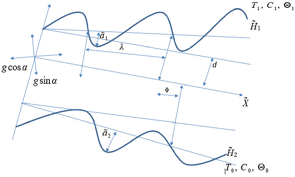
Figure 1: Flow geometry of the physical model
The equation of continuity, momentum, temperature, fraction of nanoparticles and the solute concentration of an incompressible fluid for two-dimensional cases is given as
In the above equations
Defining the subsequent dimensionless quantities
In above dimensionless quantities
By using Eq. (6), Eq. (13) is automatically satisfied and Eqs. (7)–(12) for stream function
Now using supposition of long wavelength and low number of Reynolds, the Eqs. (13)–(17) becomes
Eliminate pressure from Eqs. (18) and (19) we get
where
and
In wave frame the boundary conditions regarding stream function
The exact solution of the volume fraction of nanoparticles which satisfies the relevant condition (28) is described as
The exact solution of the solutal (species) concentration which satisfies the relevant condition (29) is described as
The exact solution of temperature which satisfies the relevant condition (27) is described as
where
The differential Eqs. (19) and (24) are non-linear so it is difficult to find exact solutions to these equations. So regular perturbation technique is used for finding the solutions of Eqs. (19) and (24). Expand now
With assistance from Eqs. (34)–(36) into Eqs. (19), (24) and (26) combining like powers of
System of order
System of order
4.1 Solution for Zeroth Order System
Solution of Eq. (37) that satisfies the boundary conditions (39)–(42) is described as follows:
The pressure gradient for this order is described as
where
4.2 Solution for First Order System
Using solution zero-order (49) into (43), the solution of Eq. (43) which satisfies the boundary conditions (45)–(48) is described as follows:
The pressure gradient for this order is described as
where
Now for small parameter
Defining
For average pressure increase the non-dimensional expression is given as follows:
The expression (in non-dimensional form) for the considered wave forms is defined as follows:
1. Multisinusoidal wave
2. Triangular wave
3. Trapezoidal wave
To interpret the results quantitatively we consider the instantaneous volume flow rate
To observe the graphical outcomes of concentration, temperature, nanoparticle fraction, pressure gradient, pressure rise and streamlines Figs. 2–11 are displayed. The temperature profile effect is plotted for the different values of Nb and NTC in Figs. 2a and 2b. It is seen in Fig. 2a that temperature profile behaviour decreases with increasing Nb values. This is because temperature exhibits a direct relationship with Nb. In Fig. 2b the temperature profile show opposite effect as compared with Nb. Here temperature effects increases with increasing NTC values. Fig. 3 shows the impact of Nt and NCT on concentration profile. It is shown in Figs. 3a and 3b that concentration profile increases with increasing Nt and NCT values. This is due to the direct relationship of concentration with Nt and NCT. To view the impact of nanoparticle fraction on Nb, Nt and NTC Figs. 4a–4c are plotted. It is shown in Fig. 4 that behavior of nanoparticle fraction decreases because of the increasing values of Nb and NTC (see Figs. 4a and 4c), whereas the behaviour of nanoparticle fraction is quite opposite for Nt. In this case nanoparticle fraction increases due to the increasing Nt values.
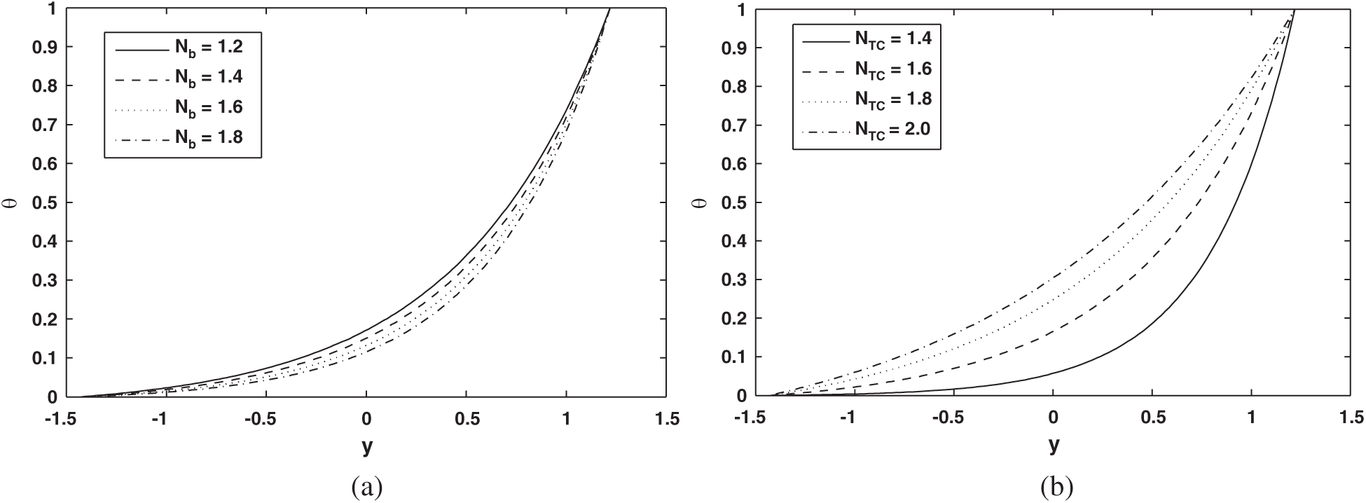
Figure 2: (a) Profile of temperature (
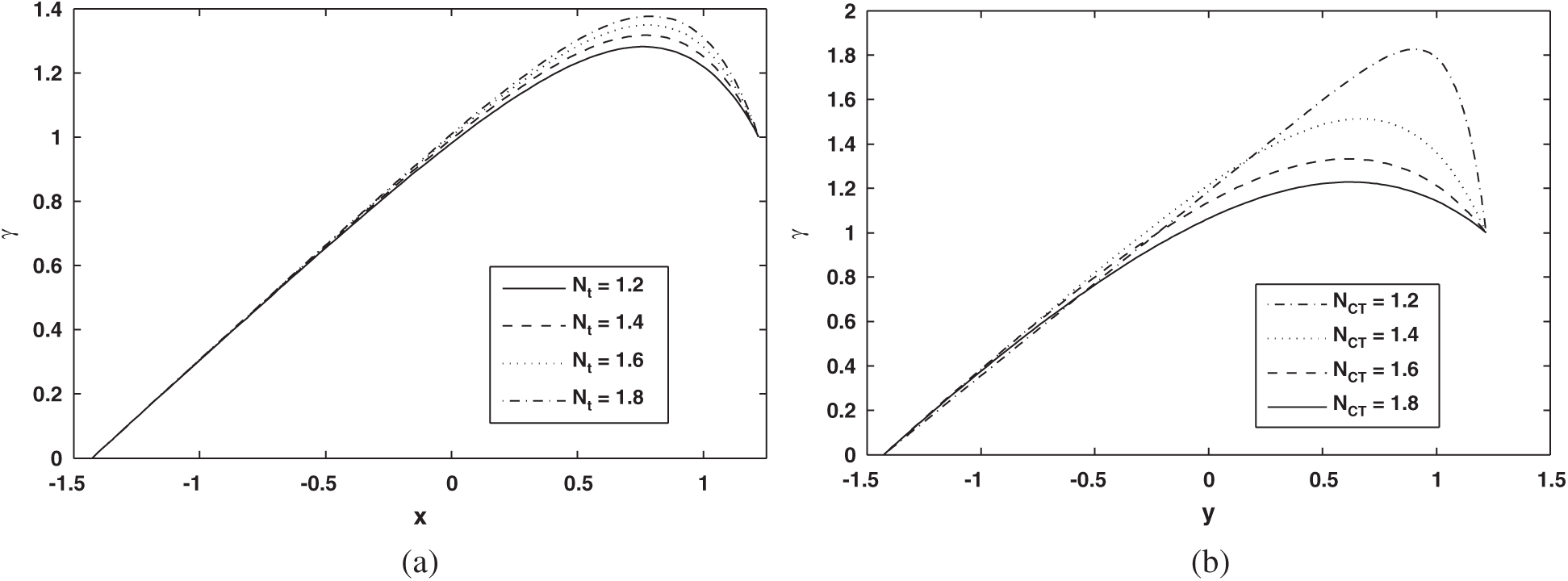
Figure 3: (a) Profile of Solutal concentration
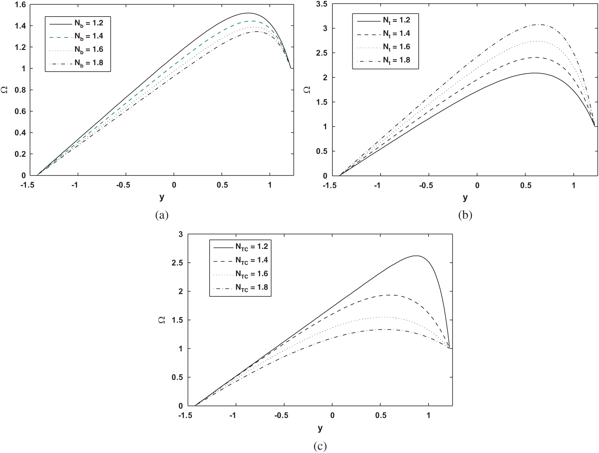
Figure 4: (a) Profile of Nanoparticle fraction
To study the graphical results of pressure, rise Figs. 5a–5d are plotted. As it turns out in Figs. 5a and 5b that pressure rise decreases within the regions where
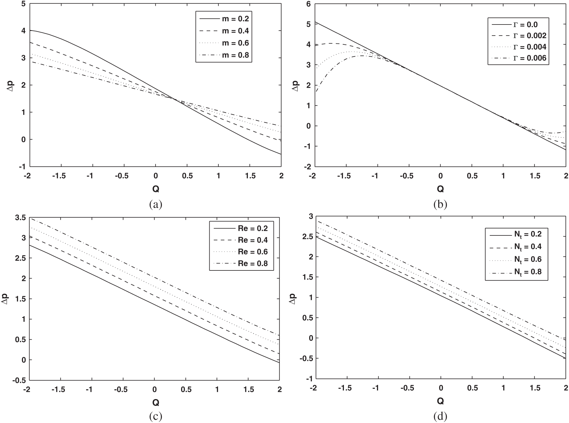
Figure 5: (a) Pressure rise over one wavelength (
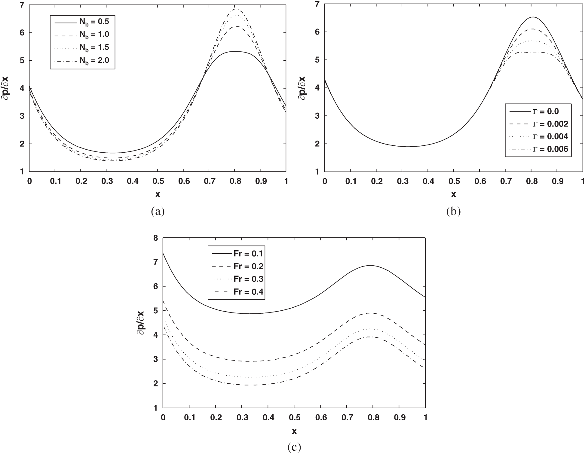
Figure 6: (a) Pressure gradient
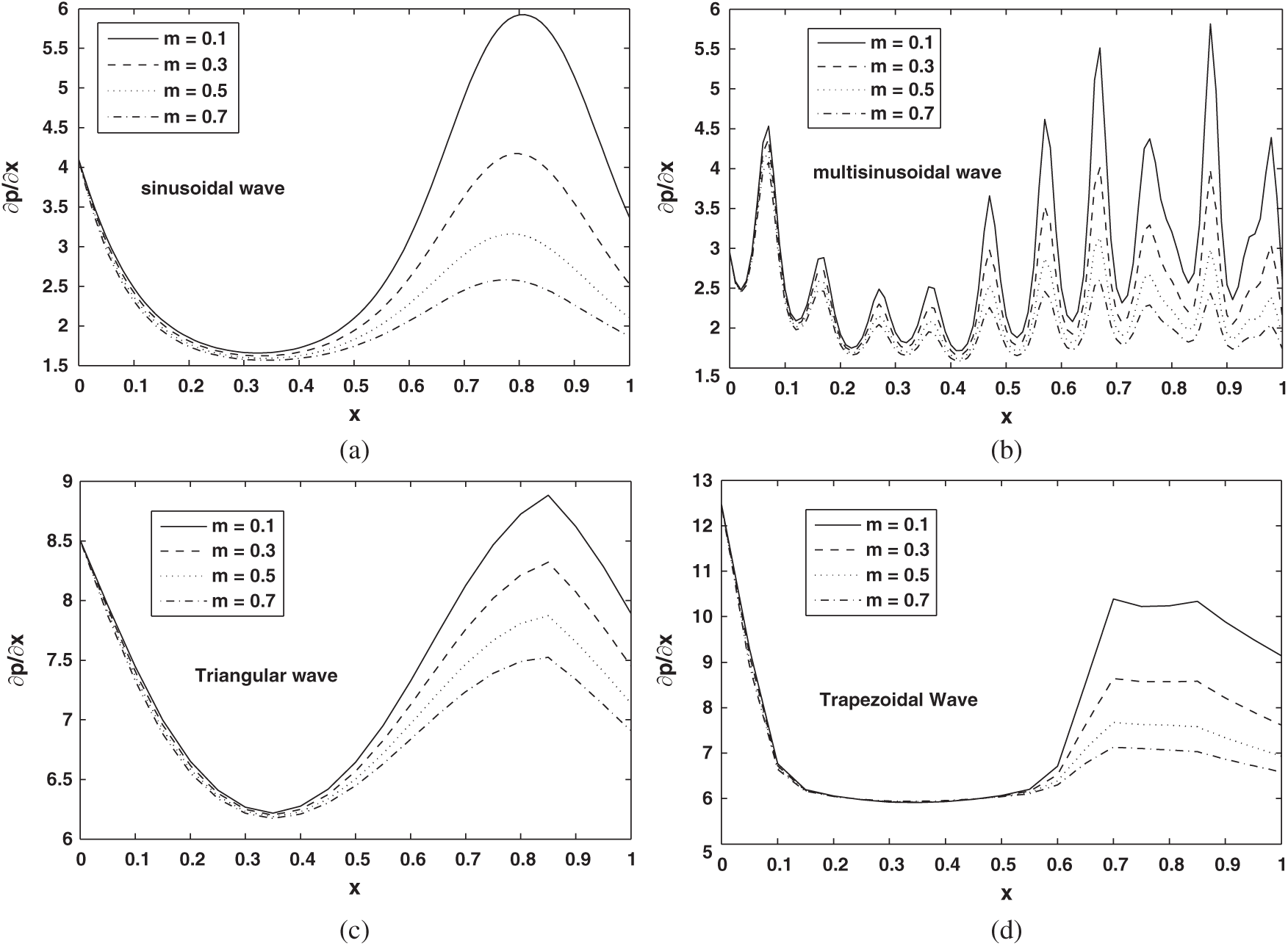
Figure 7: (a–d): Pressure gradient (dp/dx) against axial distance (x) for different wave shapes
For studying the phenomenon of trapping Figs. 8–11 are plotted. Streamlines for the different values of NCT and m are displayed in Figs. 8 and 9. It shows up in Figs. 8 and 9 that the size and number of the trapped bolus are increased by rising values of NCT and m. Fig. 10 is plotted to observe the streamlines pattern of the streamlines for different Nb values. Number of trapping bolus is observed to decrease by increasing Nb values. Patterns of streamlines for various wave types are shown in Figs. 11a and 11b.
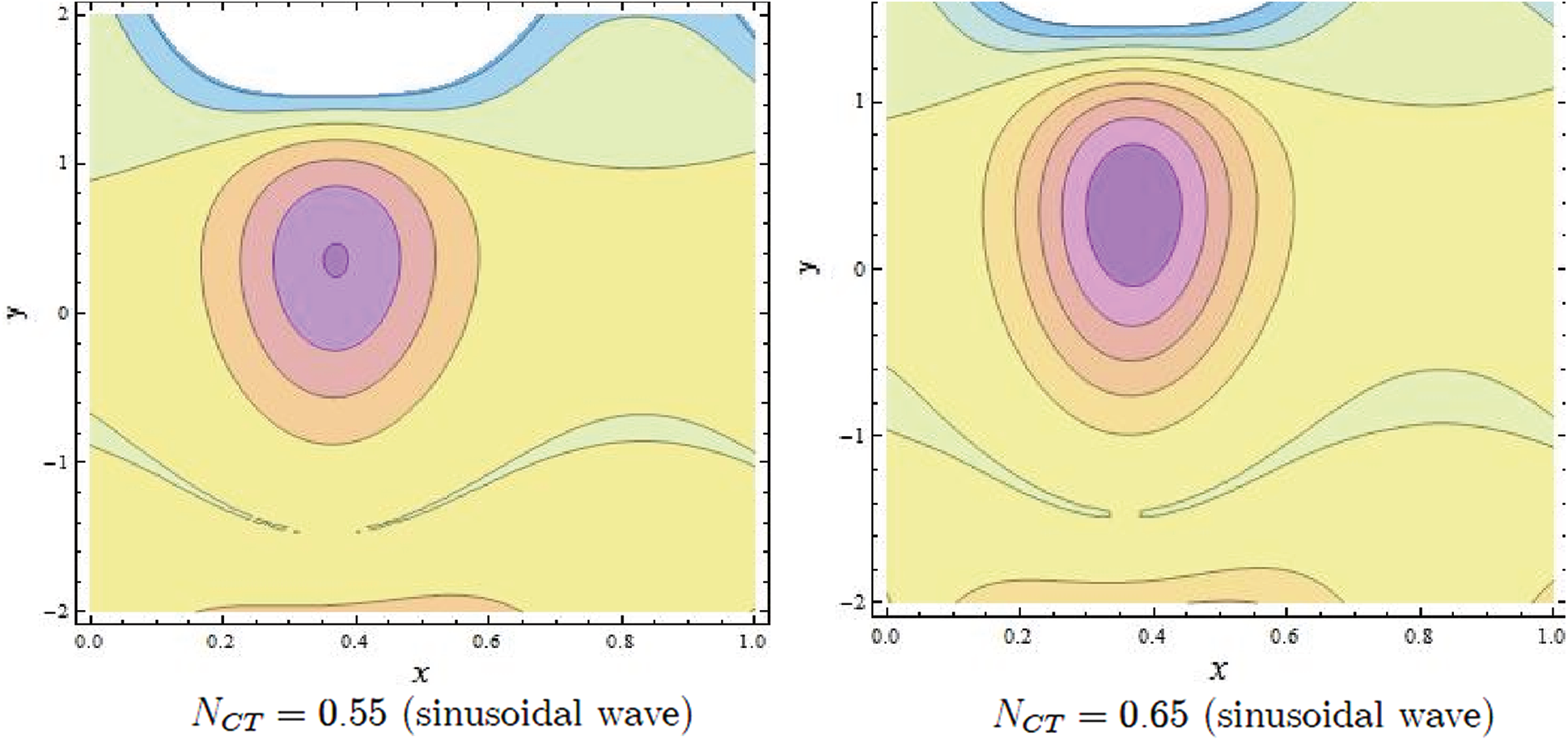
Figure 8: Streamlines of NCT
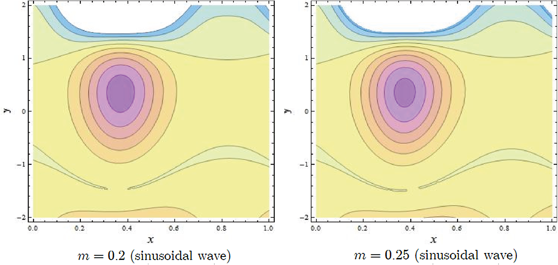
Figure 9: Streamlines of m
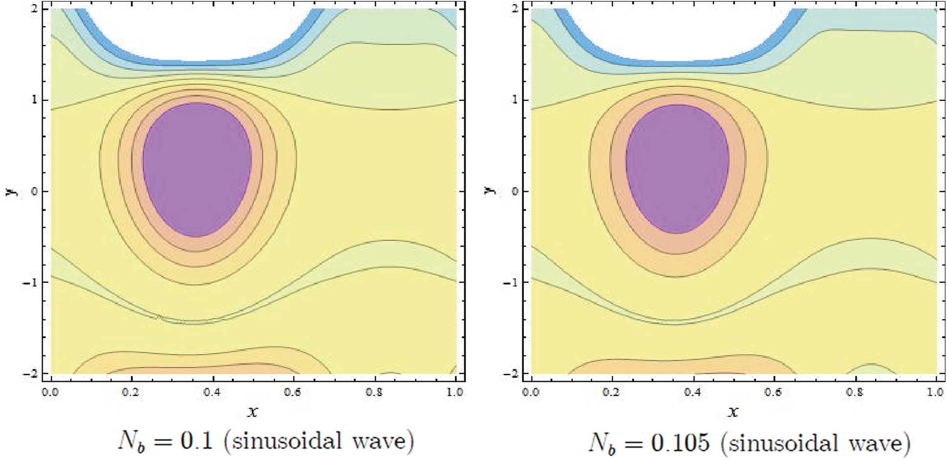
Figure 10: Streamlines of Nb
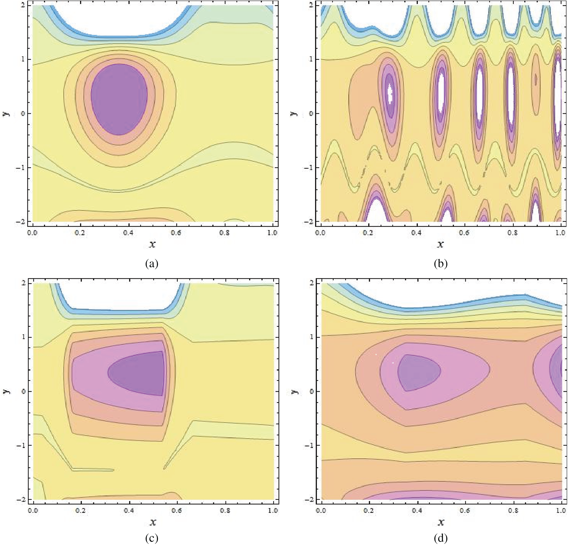
Figure 11: (a–d): Streamlines of different wave shapes
This article highlights the hybrid effects of thermal and concentration convection on peristaltic pumping of fourth grade nanofluids in an inclined tapered channel. The mathematical modelling of the fourth grade nanofluids is given along with thermal and concentration convection. Analytical technique is used to solve the differential equations that are strongly nonlinear in nature. Exact solutions of temperature, volume fraction of nanoparticles, and concentration are explored. The key finding can be encapsulated as follows:
• The temperature profile behaviour decreases with increasing Nb values and increases with increasing NTC values.
• The concentration profile increases with increasing Nt and NCT values.
• The behaviour of nanoparticle fraction decreases because of the increasing values of Nb and NTC, whereas the behavior of nanoparticle fraction is quite opposite for Nt.
• The behaviour of pressure gradient decreases due to the increasing values of Fr.
• The size and number of the trapped bolus are increased by rising values of NCT and m.
Funding Statement: The authors received no specific funding for this study.
Conflicts of Interest: The authors declare that they have no conflicts of interest to report regarding the present study.
1. Latham, T. W. (1966). Fluid motion in a peristaltic pump (Master Thesis). MIT, Cambridge. [Google Scholar]
2. Shapiro, A. H., Jaffrin, M. Y., Weinberg, S. L. (1969). Peristaltic pumping with long wavelengths at low Reynolds number. Journal of Fluid Mechanics, 37, 799–825. [Google Scholar]
3. Fung, Y. C., Yih, C. S. (1968). Peristaltic transport. Journal of Applied Mechanics, 35(4), 669–675. DOI 10.1115/1.3601290. [Google Scholar] [CrossRef]
4. Bhatti, M. M., Zeeshan, A., Tripathi, D., Ellahi, R. (2018). Thermally developed peristaltic propulsion of magnetic solid particles in Biorheological fluids. Indian Journal of Physics, 92(4), 423–430. DOI 10.1007/s12648-017-1132-x. [Google Scholar] [CrossRef]
5. Kothandapani, M., Pushparaj, V., Prakash, J. (2018). Effect of magnetic field on peristaltic flow of a fourth-grade fluid in a tapered asymmetric channel. Journal of King Saud University–Engineering Sciences, 30(1), 86–95. DOI 10.1016/j.jksues.2015.12.009. [Google Scholar] [CrossRef]
6. Ellahi, R., Hussain, F., Ishtiaq, F., Hussain, A. (2019). Peristaltic transport of Jeffrey fluid in a rectangular duct through a porous medium under the effect of partial slip: An application to upgrade industrial sieves/filters. Pramana, 93(3), 34. DOI 10.1007/s12043-019-1781-8. [Google Scholar] [CrossRef]
7. Akram, S., Mekheimer, K. S., Abd Elmaboud, Y. (2018). Particulate suspension slip flow induced by peristaltic waves in a rectangular duct: Effect of lateral walls. Alexandria Engineering Journal, 57(1), 407–414. DOI 10.1016/j.aej.2016.09.011. [Google Scholar] [CrossRef]
8. Riaz, A., Zeeshan, A., Ahmad, S., Razaq, A., Zubair, M. (2019). Effects of external magnetic field on non-Newtonian two phase fluid in an annulus with peristaltic pumping. Journal of Magnetics, 24(1), 1–8. DOI 10.4283/JMAG.2019.24.1.062. [Google Scholar] [CrossRef]
9. Haider, S., Ijaz, N., Zeeshan, A., Li, Y. Z. (2019). Magneto-hydrodynamics of a solid-liquid two-phase fluid in rotating channel due to peristaltic wavy movement. International Journal of Numerical Methods for Heat & Fluid Flow, 30(5), 2501–2516. DOI 10.1108/HFF-02-2019-0131. [Google Scholar] [CrossRef]
10. Riaz, A., Ellahi, R., Bhatti, M. M., Marin, M. (2019). Study of heat and mass transfer in the Eyring–Powell model of fluid propagating peristaltically through a rectangular complaint channel. Heat Transfer Research, 16(16), 1539–1560. DOI 10.1615/HeatTransRes.2019025622. [Google Scholar] [CrossRef]
11. Eijkle, J. C. T., van der Berg, A. (2005). Nanofluidics: What is it and what can we expect from it? Microfluidics and Nanofluidics, 1(3), 249–267. DOI 10.1007/s10404-004-0012-9. [Google Scholar] [CrossRef]
12. Choi, S. U. S. (1995). Enhancing thermal conductivity of fluid with nanoparticles. In: Siginer, D. A., Wang, H. P. (Eds.) Developments and applications of non-newtonian flows, vol. 66, pp. 99–105. New York: ASME. [Google Scholar]
13. Masuda, H., Ebata, A., Teramae, K., Hishinuma, N. (1993). Alteration of thermal conductivity and viscosity of liquid by dispersing ultra-fine particles. Netsu Bussei, 7(4), 227–233. DOI 10.2963/jjtp.7.227. [Google Scholar] [CrossRef]
14. Buongiorno, J., Hu, W. (2005). Nanofluid coolants for advanced nuclear power plants. Proceedings of ICAPP, vol. 5, no. 5705, pp. 15–19, Seoul. [Google Scholar]
15. Buongiorno, J. (2006). Convective transport in nanofluids. Journal of Heat Transfer, 128(3), 240–250. DOI 10.1115/1.2150834. [Google Scholar] [CrossRef]
16. Kothandapani, M., Prakash, J. (2015). Effect of radiation and magnetic field on peristaltic transport of nanofluids through a porous space in a tapered asymmetric channel. Journal of Magnetism and Magnetic Materials, 378(1), 152–163. DOI 10.1016/j.jmmm.2014.11.031. [Google Scholar] [CrossRef]
17. Awais, M., Farooq, S., Hayat, T., Ahmad, B. (2017). Comparative study of silver and copper water magneto nanoparticles with homogeneous-heterogeneous reactions in a tapered channel. International Journal of Heat and Mass Transfer, 115, 108–114. DOI 10.1016/j.ijheatmasstransfer.2017.07.129. [Google Scholar] [CrossRef]
18. Prakash, J., Tripathi, D., Triwari, A. K., Sait, S. M., Ellahi, R. (2019). Peristaltic pumping of nanofluids through tapered channel in porous environment: Applications in blood flow. Symmetry, 11(7), 868. DOI 10.3390/sym11070868. [Google Scholar] [CrossRef]
19. Kothandapani, M., Prakash, J. (2015). Effects of thermal radiation parameter and magnetic field on the peristaltic motion of Williamson nanofluids in a tapered asymmetric channel. International Journal of Heat and Mass Transfer, 81, 234–245. DOI 10.1016/j.ijheatmasstransfer.2014.09.062. [Google Scholar] [CrossRef]
20. Ellahi, R., Zeeshan, A., Hussain, F., Asadollahi, A. (2019). Peristaltic blood flow of couple stress fluid suspended with nanoparticles under the influence of chemical reaction and activation energy. Symmetry, 11(2), 276. DOI 10.3390/sym11020276. [Google Scholar] [CrossRef]
21. Riaz, A., Khan, S. U., Zeeshan, A., Khan, S. U., Hassan, M. et al. (2020). Thermal analysis of peristaltic flow of nanosized particles within a curved channel with second-order partial slip and porous medium. Journal of Thermal Analysis and Calorimetry, 143(3), 1997–2009. DOI 10.1007/s10973-020-09454-9. [Google Scholar] [CrossRef]
22. Akram, S. (2016). Nanofluid effects on peristaltic transport of a fourth-grade fluid in the occurrence of inclined magnetic field. Scientia Iranica, 23(3), 1502–1516. DOI 10.24200/sci.2016.3914. [Google Scholar] [CrossRef]
23. Akbar, N. S. (2014). Metallic nanoparticles analysis for the peristaltic flow in an asymmetric channel with MHD. IEEE Transactions on Nanotechnology, 13(2), 357–361. DOI 10.1109/TNANO.2014.2304362. [Google Scholar] [CrossRef]
24. Nadeem, S., Riaz, A., Ellahi, R., Akbar, N. S. (2014). Mathematical model for the peristaltic flow of Jeffrey fluid with nanoparticles phenomenon through a rectangular duct. Applied Nanoscience, 4(5), 613–624. DOI 10.1007/s13204-013-0238-5. [Google Scholar] [CrossRef]
25. Zeeshan, A., Ellahi, R., Masood, F., Hussain, F. (2019). Numerical study on bi-phase coupled stress fluid in the presence of hafnium and metallic nanoparticles over an inclined plane. International Journal of Numerical Methods for Heat and Fluid Flow, 29(8), 2854–2869. DOI 10.1108/HFF-11-2018-0677. [Google Scholar] [CrossRef]
26. Ellahi, R., Raza, M., Akbar, N. S. (2017). Study of peristaltic flow of nanofluid with entropy generation in a porous medium. Journal of Porous Media, 20(5), 461–478. DOI 10.1615/JPorMedia.v20.i5.70. [Google Scholar] [CrossRef]
27. Mosayebidorcheh, S., Hatami, M. (2018). Analytical investigation of peristaltic nanofluid flow and heat transfer in an asymmetric wavy wall channel (Part I: Straight channel). International Journal of Heat and Mass Transfer, 126(3), 790–799. DOI 10.1016/j.ijheatmasstransfer.2018.05.080. [Google Scholar] [CrossRef]
28. Hayat, T., Iqbal, R., Tanveer, A., Alsaedi, A. (2016). Influence of convective conditions in radiative peristaltic flow of pseudoplastic nanofluid in a tapered asymmetric channel. Journal of Magnetism and Magnetic Materials, 408, 168–176. DOI 10.1016/j.jmmm.2016.02.044. [Google Scholar] [CrossRef]
29. Hayat, T., Iqbal, R., Tanveer, A., Alsaedi, A. (2016). Mixed convective peristaltic transport of Carreau–Yasuda nanofluid in a tapered asymmetric channel. Journal of Molecular Liquids, 223(2014), 1100–1113. DOI 10.1016/j.molliq.2016.08.003. [Google Scholar] [CrossRef]
30. Hussain, F., Ellahi, R., Zeeshan, A., Vafai, K. (2018). Modelling study on heated couple stress fluid peristaltically conveying gold nanoparticle through coaxial tube: A remedy for gland tumor and arthritis. Journal of Molecular Liquids, 268, 149–155. DOI 10.1016/j.molliq.2018.07.034. [Google Scholar] [CrossRef]
31. Akbar, N. S. (2014). Double-diffusive natural convective peristaltic flow of a Jeffrey nanofluid in a porous channel. Heat Transfer Research, 45(4), 293–307. DOI 10.1615/HeatTransRes.2013006995. [Google Scholar] [CrossRef]
32. Asha, S. K., Sunitha, G. (2020). Thermal radiation and hall effects on peristaltic blood flow with double diffusion in the presence of nanoparticles. Case Studies in Thermal Engineering, 17(4), 100560. DOI 10.1016/j.csite.2019.100560. [Google Scholar] [CrossRef]
33. Kuznetsov, A. V., Nield, D. A. (2011). Double-diffusive natural convective boundary-layer flow of a nanofluid past a vertical plate. International Journal of Thermal Sciences, 50(5), 712–717. DOI 10.1016/j.ijthermalsci.2011.01.003. [Google Scholar] [CrossRef]
34. Akram, S., Razia, A., Farkhanda, A. (2020). Effects of velocity second slip model and induced magnetic field on peristaltic transport of non-Newtonian fluid in the presence of double-diffusivity convection in nanofluids. Archive of Applied Mechanics, 90(7), 1583–1603. DOI 10.1007/s00419-020-01685-4. [Google Scholar] [CrossRef]
35. Sharma, A., Tripathi, D., Sharma, R. K., Tiwari, A. K. (2019). Analysis of double diffusive convection in electroosmosis regulated peristaltic transport of nanofluids. Physica A, 535, 122148. DOI 10.1016/j.physa.2019.122148. [Google Scholar] [CrossRef]
36. Narayana, M., Sibanda, P. (2012). On the solution of double-diffusive convective flow due to a cone by a linearization method. Journal of Applied Mathematics, 2012(5), 1–19. DOI 10.1155/2012/587357. [Google Scholar] [CrossRef]
37. Nield, D. A., Kuznetsov, A. V. (2011). The onset of double diffusive convection in a nanofluid layer. International Journal of Heat and Fluid Flow, 32(4), 771–776. DOI 10.1016/j.ijheatfluidflow.2011.03.010. [Google Scholar] [CrossRef]
38. Akram, S., Zafar, M., Nadeem, S. (2018). Peristaltic transport of a Jeffrey fluid with double-diffusive convection in nanofluids in the presence of inclined magnetic field. International Journal of Geometric Methods in Modern Physics, 15(11), 1850181. DOI 10.1142/S0219887818501815. [Google Scholar] [CrossRef]
39. Anwar Bég, O., Tripathi, D. (2012). Mathematica simulation of peristaltic pumping with double-diffusive convection in nanofluids a bio-nanoengineering model. Proceedings of the Institution of Mechanical Engineers, Part N: Journal of Nanoengineering and Nanosystems, 225, 99–114. [Google Scholar]
40. Alolaiyan, H., Riaz, A., Razaq, A., Saleem, N., Zeeshan, A. et al. (2020). Effects of double diffusion convection on third grade nanofluid through a curved compliant peristaltic channel. Coatings, 10(2), 154. DOI 10.3390/coatings10020154. [Google Scholar] [CrossRef]
Appendix
 | This work is licensed under a Creative Commons Attribution 4.0 International License, which permits unrestricted use, distribution, and reproduction in any medium, provided the original work is properly cited. |