Computer Modeling in Engineering & Sciences

DOI: 10.32604/cmes.2021.014199

ARTICLE

Parameters Identification of Tunnel Jointed Surrounding Rock Based on Gaussian Process Regression Optimized by Difference Evolution Algorithm

Annan Jiang*, Xinping Guo, Shuai Zheng and Mengfei Xu

Highway and Bridge Institute, Dalian Maritime University, Dalian, 116026, China
*Corresponding Author: Annan Jiang. Email: jiangannan@163.com
Received: 10 September 2020; Accepted: 04 February 2021

1  Introduction

The ability to identify the mechanical parameters of surrounding rock of a tunnel based on field monitoring information is crucial for the construction mechanics in the geotechnical engineering field. The identification of surrounding rock parameters is also called the back analysis. Using different monitoring information, the stress back analysis, displacement back analysis, and mixed back analysis can be concocted. The combined displacement–stress back analysis method has been widely applied to geotechnical engineering [1].

Different constitutive models can describe a different mechanical behavior of surrounding rock. In the 1970s, a surrounding rock of a tunnel was simplified into a uniform elastic constitutive model, and the parameter inversion was mainly to identify the elastic modulus. Kavanagh et al. [2] presented a finite element method for inverting the elastic modulus of elastic solids. Kirsten [3] proposed the back analysis method of measured deformation at the conference of geotechnical investigation in Johannesburg. With the development of computational mechanics, the parameter identification methods of more complex constitutive models have attracted great attention of scholars [4]. Gioda et al. [5,6] studied the back analysis methods of the elastic-plastic model. Gao et al. [7] developed a displacement back analysis algorithm, considering the time-dependent effect of the rock mass. Vardakos et al. [8] presented a numerical back-analysis of the response of the Shimizu Tunnel No. 3 during the construction process based on distinct element modeling. It is worth noting that most of the studies on the back analysis have been limited to two-dimensional models. However, it is very common for a tunnel to cross the weak joints, so the isotropic homogeneous model cannot accurately describe the mechanical behavior of the surrounding rock. Recently, the anisotropic elastoplastic constitutive model called the ubiquitous-joint model has been proposed. This model can reflect how a weak plane affects the rock mass deformation after yielding. Das et al. [9,10] and Ismael et al. [11] studied the ubiquitous-joint model in different engineering fields.

Rich research results have been achieved in the field of tunnel surrounding rock parameter identification. However, limited studies have been conducted using the ubiquitous-joint model and three-dimensional (3D) model. The main reason is that the complex constitutive model and 3D numerical calculation are time-consuming, which makes the parameters identification more difficult [12,13]. In order to improve the computing speed, more and more evolutionary intelligent optimization algorithms, including the genetic algorithm (GA) [14], evolution strategy algorithm (ESA) [15], and particle swarm optimization (PSO) [16,17], have been combined with numerical algorithms for back analysis. Furthermore, the nonlinear respond surface methodology (RSM) has been employed to map the nonlinear relation between the mechanical parameters and displacement of surrounding rock. The multivariate adaptive regression splines and logistic regression [18], artificial neural network (ANN) [19,20], support vector machine (SVM) [21], and other algorithms have been used to construct the RSM model. However, due to the complexity of parameters identification of jointed surrounding rock, there are certain problems in the field of the mechanical parameters identification of surrounding rock of a tunnel, and they can be summarized as follows:

(1) Optimization algorithms have certain shortcomings; for instance, the GA includes encoding and decoding, and its operation is complex; the PSO algorithm is relatively simple, but its mathematical theory is not strict enough. The optimization algorithms can also be limited to the local optimal problem and become precocious easily [22].

(2) The ANNs are based on the empirical risk minimization and have the disadvantages of requiring a large amount of training data, over-learning, and poor generalization ability.

(3) Although the SVM can be used for the sequential minimum optimization and other fast learning algorithms, its operating speed is slow when the number of learning samples is too large, and the estimated output is not probabilistic [23]. Therefore, it is necessary to explore other machine learning-based algorithms and intelligent optimization methods for ubiquitous-joint model parameter identification.

The Gaussian process (GP) regression combines nuclear machine learning and Bayesian reasoning, which provides many outstanding advantages, such as flexible non-parametric inference, adaptive parameter acquisition, and simple implementation process [24,25]. Difference evolution (DE) optimization has good robustness, strong global search ability, and simple structure, and it is not dependent on the characteristic information on the problem itself, which makes it be suitable for solving all types of complex optimization problems [26,27]. Therefore, the aim of this paper is to introduce the GP and DE to the surrounding rock parameter identification based on a 3D model and a ubiquitous-joint model. In this work, the GP is used to reflect the nonlinear relationship between the jointed parameters and displacement and stress of surrounding rock. In addition, the 3D numerical simulation and orthogonal design are conducted to obtain the training data samples. In order to improve the mapping effect, the super-parameters of the GP model are optimized by the DE algorithm. Then, the trained GP model is integrated into the DE algorithm to identify the parameters of the jointed surrounding rock. Finally, the proposed method is verified by an experiment with the Dadongshan tunnel of Dalian city, China, and the algorithm performances are discussed in detail. The proposed method realizes the back analysis of the joint parameters of the surrounding rock in Dadongshan tunnel and effectively guides the safe construction.

The remainder of this paper is organized as follows. In Section 2, the background of back analysis of tunnel surrounding rock is introduced. In Section 3, the parameter identification method based on the GP-DE is introduced. In Section 4, the application of the proposed method in engineering is presented. In Section 5, the parameters of GP and DE are analyzed. Finally, conclusions are drawn in Section 6.

2  Background of Back Analysis of Tunnel Surrounding Rock

With the rapid development of computational mechanics and computer technology, numerical analysis methods have begun to be applied in the field of rock mechanics research, with strong universal applicability. However, the numerical analysis method is under a strong dependence on the selection of model parameters. The accuracy of the parameters will directly affect the final calculation results. How to obtain surrounding rock parameters effectively and reasonably has become a key issue in tunnel engineering calculations [13]. For these problems, the method of back-analyzing and calculating the equivalent parameters of surrounding rock by using field monitoring data has become an effective means to solve such problems [4]. Back analysis is a method of calculating geotechnical parameters or initial ground stress of geotechnical engineering based on field observation data and through mechanical inversion analysis model. From 1970s to now, scholars have begun back analysis research in geotechnical engineering and got rich relatively researching results. The classification of back analysis methods is shown in Fig. 1.

According to different kinds of monitored information, back analysis is divided into stress back analysis [28], displacement back analysis [13] and mixed back analysis [27]. Displacement back analysis has problems such as lagging and being affected by three-dimensional spatial effects [29]. Stress back analysis is also insensitive to elastic modulus and other reflections, which may cause the back analysis to have a non-unique solution. Therefore, the mixed back analysis can make full use of monitoring information and improve the accuracy of parameter inversion. According to calculation methods, the analytical method and the numerical method are distinguished. Moreover, numerical method is divided into reverse solving method and forward solving method. The reverse solving method is based on inverse process of finite element analysis, and the advantage is that the analysis efficiency is very high, but it is only suitable for relatively simple models [30]. The forward solving method is to use the forward solver and certain optimization techniques to can carry out complex calculation procedures. Therefore, the analytical method and reverse solving method require a lot of simplification of tunnel engineering, which is limited to the actual tunnel, while forward solving method has more powerful adaptability and is increasingly widely used. The optimization algorithms play a key role in the back analysis method. Early time the traditional algorithms were adopted such as the golden section method, the simplex method, and the Newton method [2–5]. Since the 1990s, modern computational intelligence methods represented by genetic algorithms and neural network methods have been applied in geotechnical engineering and have continued to develop.

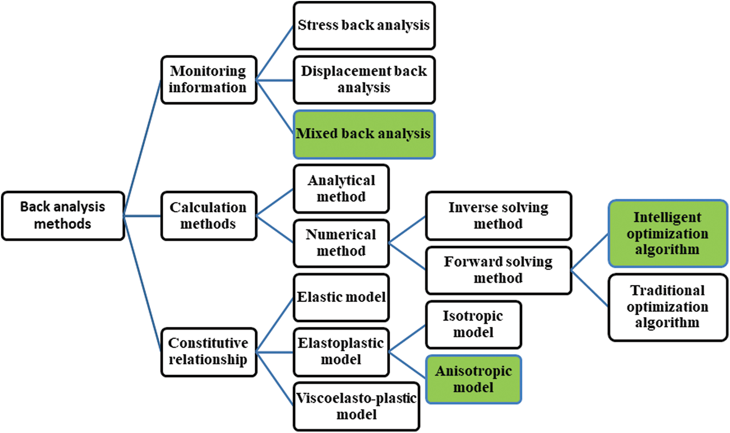
Figure 1: Classification of geotechnical back analysis

The selection of constitutive model is the basis for determining the accuracy of numerical calculation of the tunnel surrounding rock. The constitutive models used in the back analysis are generally divided into elastic models [2,3], elastoplastic models [5,6] and viscoelastic models [7]. Furthermore, the elastoplastic models are divided into isotropic models and anisotropic models. The actual rock mass includes various discontinuous bodies or even broken bodies, so the conventional models of elasticity or isotropic elastoplasticity cannot reflect the characteristics of rock mass well. The ubiquitous joint model is an excellent anisotropic which is to use the form of traditional strength criteria, introduce a tensor composed of the shear strength (or tensile strength) in the main direction of the material, and find the most likely failure surface under certain stress conditions [9,10,31].

The trend of back analysis is to adopt more complex constitutive models which can describe the actual rock mass, however, there no report about back analysis of ubiquitous joint model parameters can be seen now. The numerical calculation based on ubiquitous joint model concerns more parameters, the relation between parameters and monitoring data is more complex. Therefore the general back analysis methods are limited. The intelligent optimization algorithms with better robust and the RSM with better nonlinear fitting capabilities should be adopted. Therefore, this study proposes the new GP-DE algorithm for ubiquitous-joint model parameters inversion, and comprehensively utilizes displacement and stress information, finally provides an effective back analysis method for the surrounding jointed rock of tunnel engineering.

3  The Parameters Identification Method Based on GP-DE

3.1 Ubiquitous-Joint Model of Rock Mass Engineering

Because of the excavation unloading effect, the surrounding rock deformation toward the empty surface increases continuously, which causes that part of the surrounding rock to change from the elastic stage to the plastic stage, and the loose zone occurs. In this process, the joints combined with the rock matrix of the surrounding rock all play important roles, which can be expressed by a ubiquitous-joint model. The rock matrix and joints considered in the ubiquitous-joint model satisfy the Mohr–Coulomb yielding criteria. The direction of the joint surface and the stress state can be represented by the three directions (x, y, z) in the overall Cartesian coordinate system. When selecting a set of joints for analysis, the normal direction of the joint surface is the σf-axis, the projection of the joint dip on the joint plane is the σn-axis, and the horizontal direction id the y′-axis. The local coordinate system established by the right-hand rule and configuration of ubiquitous joints in the rock mass is shown in Fig. 2.

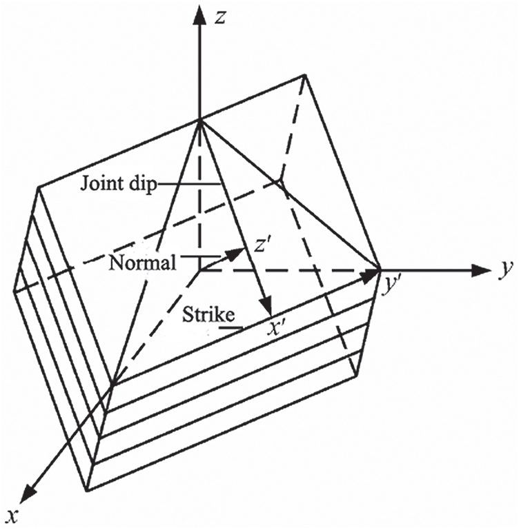
Figure 2: Configuration of ubiquitous joints in rock mass

Therefore, the relationship between the stress tensors σ and σ′ that correspond to the global and local coordinate systems, respectively, can be expressed as:

[σ′]=[C]T[σ][C],(1)

where [C] denotes the directional tensor and the cosine of the angle between the local coordinate system and the global coordinate system in the three directions, and it is defined as:

C=[cos(x′,x)cos(x,y)cos(x′,z)cos(y′,x)cos(y′,y)cos(y′,z)cos(z′,x)cos(z′,y)cos(z′,z)],(2)

Further, the shear yield criterion and tensile yield criterion of joints can be respectively expressed as follows:

fs=τ+σ3′3′tanϕj-cj=0,(3)

ft=σ3′3′-σjt=0,(4)

where cj represents the cohesion, ϕj denotes the rock inner friction angle, σjt is tensile strength, τ represents the shear stress on the joint plane, and σ3′3′ is the normal stress of a joint in the local coordinate system. The shear and tensile plastic flow of the joint surface are expressed as functions gs and gt. The potential function gs represents the uncorrelated flow rule, and it is expressed as follows:

gs=τ+σ3′3′tanψj,(5)

where ψj denotes the weak-plane dilation angle.

The potential function gt corresponds to the associated flow rule, and it is defined as follows:

gt=σ3′3′,(6)

Based on Eqs. (1)–(6), the joint parameters include cj, ϕj, σjt, and ψj. When the joint dip angle and joint dip direction are considered, there are six parameters. To simplify the presentation, the mentioned six parameters are denoted as follows: joint surface cohesion as Jcoh, joint surface friction angle as Jfric, joint surface tensile strength as Jten, joint surface dilatation angle as Jdila, joint surface dip as Jdip, and joint surface dip angle as Jdd.

3.2 The Problem of Jointed Rock Parameters Identification

The identification of the jointed surrounding rock parameters is essentially an optimization problem. The upper and lower limits are defined based on the specific physical meaning of model parameters. Assuming that there are m observed values in the region, the constrained optimization problem can be expressed as:

minE(x1,x2,…,xN)= min(1m∑k-1m|Yk0-Yk|)xka≤xk≤xkb(k=1,2,…,N),(7)

where Yk0 denotes the measured displacement or stress, Yk represents the calculated displacement or stress, m is the number of observed values, xk is the surrounding joint rock parameter, N denotes the number of parameters, and xka and xkb are the upper and lower limits of the surrounding joint rock parameters, respectively. The identification process is shown in Fig. 3.

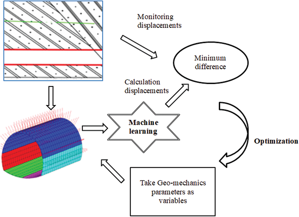
Figure 3: Geotechnical engineering parameters identification process

As shown in Fig. 3, the parameters process needs many forward calculations and consumes much time when the 3D numerical simulation is used. Therefore, the GP is used to construct the responding surface of jointed parameters and displacements of the surrounding rock.

3.3 The GP Respond Surface Optimized by DE

The GP is a fast developing machine learning method that has good nonlinear performance, but suffers from the problems of high dimension, and small sample regression. According to [23], the brief introduction of GP is as follows:

Assume X=[x1,x2,…,xn] is the d×n input matrix, and y=[y1,y2,…,yn] is the output vector, then the training dataset can be expressed as {X, y}; thus, the standard linear regress model with the Gaussian white noise can be expressed as:

yi=f(xi)+ε,(8)

where ε denotes an independent random variable, and ε~N(0,σn2), while σn2 represents the variance.

The prior distribution of the observed target value y can be expressed as:

y~N(0,C+σn2I),(9)

where C = C(X, X) denotes a symmetric positive definite covariance matrix of the nth order.

For the test sample (x*, y*), where x*= (x1*, x2*, x3*, …, xn*), y*= (y1*, y2*, y3*, …, yn*), the joint Gaussian prior distribution of y and y* can be obtained and expressed as:

[yy*]~N(0,[C(X,X)+σn2IC(X,x*)C(x*,X)C(x*,x*)]),(10)

where C(X,X) denotes an n×n symmetric positive definite covariance matrix, and I represents the identity matrix; C(X, x*) = C(x*, X)T is an n × 1 covariance matrix consisted of new input test points x* and all input points; C(x*, x*) is the covariance matrix consisted of new input test points x*.

When the training set D and the input value x* of a test sample are known, the GP can use the posterior probability formula to calculate the output value y* of the test sample, which be expressed as:

y*|x*,D~N(uy*,σy*2),(11)

uy*=C(x*,X)(C(X,X)+σn2I)-1y,(12)

where uy* and σy*2 denote the expectation and variance of y*, respectively.

The covariance function is used to measure the similarity degree between the training sample and prediction samples. According to Eq. (11), the kernel function of traditional machine learning can be expressed by the covariance function. The covariance function used in this work is the square exponential covariance function (SE), and it is expressed as:

kse(xp,xq)=σf2exp(−12J2‖ xp−xq ‖2)+σn2δpq,(13)

where xp and xq can represent the learning samples, prediction samples, or combinations of learning and prediction samples depending on a particular situation; J is the distance correlation between the two data points xp and xq; σf is the local correlation; σn is the standard deviation of the noise; and lastly, δpq is a sign function, and when p = q, then δpq= 0; otherwise, δpq= 1.

The GP-based surface should be trained by representative data samples before it can map the complex nonlinear relation between the jointed parameters and displacements. The data samples can be obtained by model tests, field tests, numerical simulation, and other methods. In this study, the data samples are collected using the orthogonal design, uniform design, and numerical simulation. In the GP training process, hyper-parameters σf and σn affect the GP training effect and prediction accuracy, so this process can be described as an optimization problem, which is expressed as:

minE(θ)=min(∑n−1K| GPh(θ)−YhYh |), h=1,2,…,K,(14)

where GPh(θ) and Yh denote the estimated output data of the tentative GP and the real output corresponding to the hth test sample. The test sample number is h = 1, 2,…, K; and, θ= (σf, σn) represents the hyper-parametric vector.

It is difficult to select the above parameters artificially, so in this study, an intelligent optimization algorithm DE is used to optimize θ. The DE was proposed by Stom and Price in 1995, and it has an excellent performance in solving the global minimum convergence problems and complex problems with many parameters, constraints, and objectives [25]. The DE directly converts the solution to the optimization problem into a D-dimensional solution vector, and each solution vector is the basic individual of the evolution. The basic operation of the DE algorithm includes the following four steps: (1) Initial population generation

The original population that includes the NP individuals is generated randomly and uniformly distributed in the solution space as follows:

xi,j,0=xi,jL+rand(xi,jU−xi,jL), i=1,2,⋯,NP; j=1,2,⋯,D,(15)

where rand is a random number between zero and one, and xi,jU and xi,jL are upper and lower boundary of variables, respectively.

(2) Mutation operation

For each target vector of the Gth generation xi,G, the mutation vector is defined as:

Vi,G+1=Xr1,G+F(Xr2,G-Xr3,G),(16)

where r1, r2, r3∈ [1, 2, …, NP] denote different random integers, F is the mutation factor, which is used to adjust the step amplitude of the vector difference, and it is the main control parameter whose value is between zero and one.

(3) Crossover operation

In order to increase the diversity of the population, a new test vector ui,G+1 is obtained by the hybridization of target vectors xi,G and vi,G+1 as follows:

ui,G+1={Vi,G+1,rj≤CR∥j=niXi,G,rj>CR&j≠ni,(17)

where rj∈ [0, 1] is a random number corresponding to the j; CR ∈ [0, 1] is the crossover factor, ni is a random integer having the value form the set (1, 2,…, D), which guarantees that vector vi,G+1 has at least one component of the test vector ui,G+1.

(4) Selection operation

The new generation of the population obtained by the selection operation is expressed as:

xi,G+1={ui,G+1if(f(ui,G+1)≤f(xi,G))xi,Gf(f(ui,G+1)>f(xi,G)),(18)

where f(⋅) represents the fitness function that correspond to Eq. (14). By using the DE, the GP hyper-parameters can be obtained quickly, as well as the training samples with the parameters, so the GP respond surface mapping with the input consisted of the jointed parameters, and the output consisted of displacement and stress values can be constructed.

3.4 The Parameters Identification Flowchart

Based on Eq. (7), Yk can be calculated using the GP model instead of the ubiquitous-joint model, and in that case, it is expressed by Eq. (19). Also, by using the DE algorithm, the jointed rock parameters can be identified

minE(x1,x2,…,xN)= min(1m∑j=1m|GP(x1,x2,…,xN)j0-Yj|)xka≤xk≤xkb(k=1,2,…,N),(19)

In Eq. (19), m denotes the number of key points (or measure lines), and Yj represents the monitored information of the jth key point. The flowchart of the jointed rock parameters identification is displayed in Fig. 4.

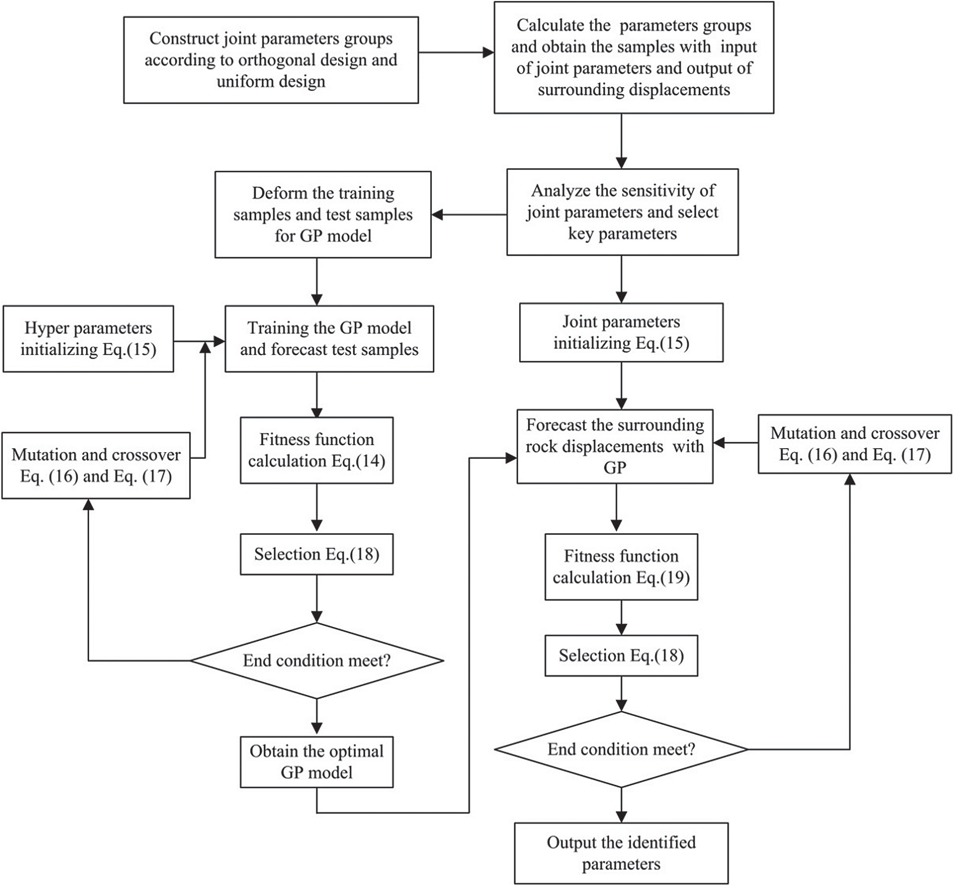
Figure 4: Flow chart of joint rock parameters identification

The specific algorithm steps are as follows:

1.    By using the orthogonal and uniform design methods, the six parameters of the joint model, including the joint surface cohesion, joint surface dilatation angle, joint surface friction angle, joint surface tensile strength, joint surface dip, and joint surface dip angle, are designed in different parameter combination schemes.

2.    For each analysis task, the training datasets that correspond to the jointed surrounding rock parameters and displacement and stress values at key points are constructed. Numerical analysis is used to calculate the dataset for each set of the orthogonal and uniformly experimental schemes. To improve the generation performance of the GP, the test dataset is selected from the training dataset and used to assess the applicability of the GP.

3.    The GP model is constructed such that to describe the nonlinear relationship between the joint parameters and key displacement and stress values. The orthogonal design samples are used to train the GP model, and the uniform design samples are used to test the GP model.

4.    The parameters of the DE-GP model, including the population size, evolutionary generation number, and hyper-parameter ranges of the GP kernel function, are initialized. Each hyper-parameter group is considered as an individual in the GP. A dataset is randomly generated in the solution space as the initial population according to Eq. (15).

5.    The operations of mutation and crossover are performed according to Eqs. (16) and (17), respectively. The GP model is trained using the hyper-parameters’ values, and the predicted values are compared with the corresponding test values. The fitness value of the current individual is evaluated by Eq. (14), and the selection operation according to Eq. (18) is adopted.

6.    If the preset termination conditions for the iteration number or the minimal error are satisfied, and the identified parameters are given, the GP training procedure terminates, and the algorithm turns to the next step; otherwise, the algorithm returns to Step 5.

7.    The parameters of the DE-GP model, including the population size, evolutionary generation number, and the parameter range for the jointed rock, are initialized. A dataset is randomly generated in the solution space as the initial population according to Eq. (15).

8.    The operations of mutation and crossover are performed according to Eqs. (16) and (17). A set of data obtained above is input to the GP model to calculate the displacement of key points. The fitness value of the current individual is evaluated by Eq. (19), and the selection operation is conducted following Eq. (18).

9.    If predefined termination conditions for the iteration number or the minimal error are satisfied, the optimal parameters are obtained; otherwise, the algorithm returns to Step 8.

4  Engineering Application

4.1 Engineering Overview

The proposed method was verified by the experiment with the Dadongshan tunnel, which is part of the Bohai Avenue Engineering of high way in Dalian city, China. It includes two super large section tunnels with a small clear distance. The lengths of the western and eastern tunnels are 1,113.8 and 1,110.3 m, respectively. The height and width of tunnel clearance are 10.1 and 18.2 m, respectively, and the maximum depth of the tunnel from the ground surface is 155 m. The minimum thickness of the rock column between the two holes is 15.9 m. The map location and field scene of the tunnel under study are shown in Fig. 5.

The regional strata were mainly thick quartz sandstone of the qiaotou formation (Qnq) of the Xihe District group of Qingbaikou series. The joints and fissures of rock mass around the construction site were developed. Four groups of main joints were found through the exploration, most of which were closed to microtensioned and not filled.

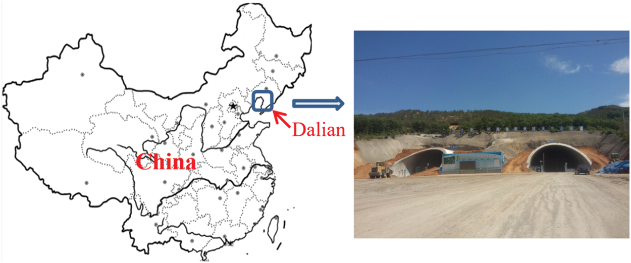
Figure 5: The location of the Dadongshan tunnel

4.2 Numerical Simulation Model

The tunnel interval mileage K7 + 620 m–K7 + 660 m, where the third group of joint faces was located, was selected as a study object. The 3D numerical model established by the geotechnical engineering software FLAC3D is shown in Fig. 6. The surrounding rock displacements and stress measurement points of the left tunnel were arranged in a way that is presented in Fig. 6. The size of the calculation model was 166 m × 80 m × 40 m. The overlying strata were converted to the equivalent loads. The constitutive model adopted the ubiquitous-joint model.

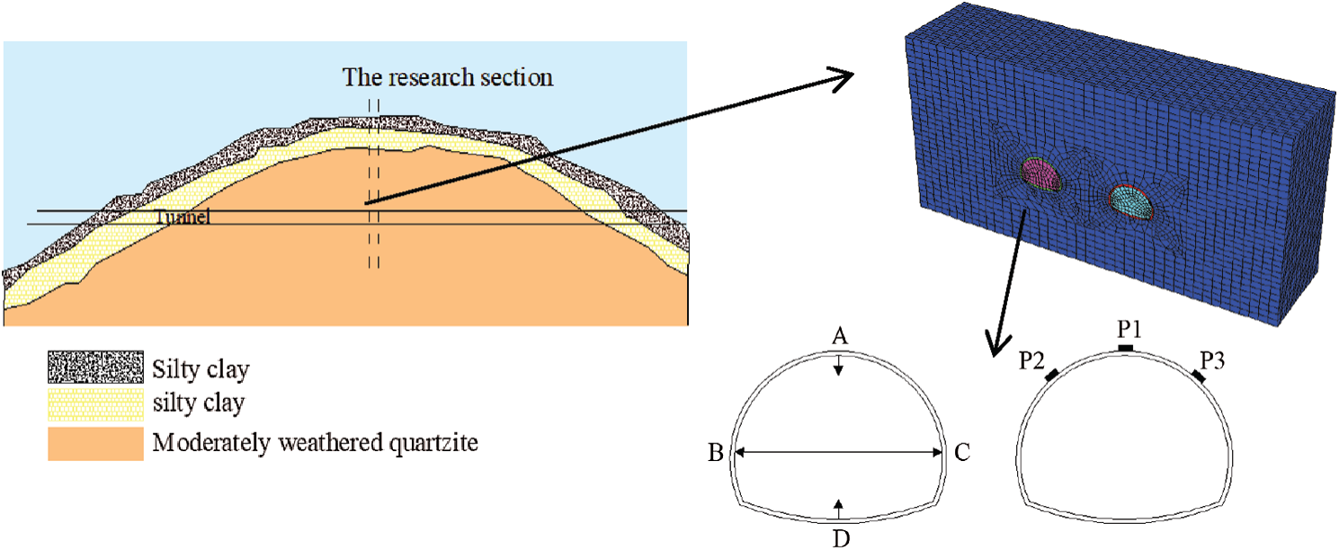
Figure 6: Tunnel numerical calculation model

The surrounding rock medium was mainly apoplexy fossil English sandstone. The parameters of the corresponding rock matrix were as follows: Young’s modulus was 1200 MPa, Poisson’s ratio was 0.2, cohesion was 1.0 MPa, and the angle of internal friction was 30∘. The left and right tunnels were constructed using the double-sided guide pit method. The excavation sections of each excavation step were staggered. The null, shell, and cable elements were adopted to simulate the excavation, lining, and bolts in the construction process, respectively. The ubiquitous-joint model parameters were considered to be identified. As mentioned in Section 3.1, the six joint parameters denoted as Jcoh, Jfric, Jten, Jdila, Jdip, Jdd, were determined based on the experience and geological prospecting data; the obtained parameters’ ranges are shown in Tab. 1. Based on the six joint parameters’ ranges, 25 orthogonal design schemes and five uniform design parameter combination schemes were generated. The monitoring points of the arch waist were B and C, and the convergence displacement of them was BC. The settlement of the top arch and the floor lifting were denoted as AZ and DZ, respectively. Three stress monitoring points were arranged on the top arch, as shown in Fig. 6. The parameters of each scheme were fed to the numerical model to conduct the numerical simulation. The orthogonal parameters schemes, uniform design parameter combination schemes, and calculated displacements are shown in Tabs. 2 and 3.

The data given in Tab. 2 were used as the training data of the GP model, and the data given in Tab. 3 were used as the test data. Following the procedure presented in Section 3.3, the response surface model of the Gaussian process was constructed, which represented the mapping of the nonlinear relationship between the jointed rock mass parameters and the corresponding displacements and stress values.

Table 1: Jointed surrounding rock parameters range

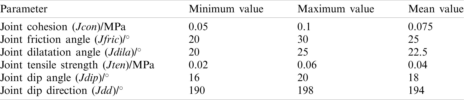
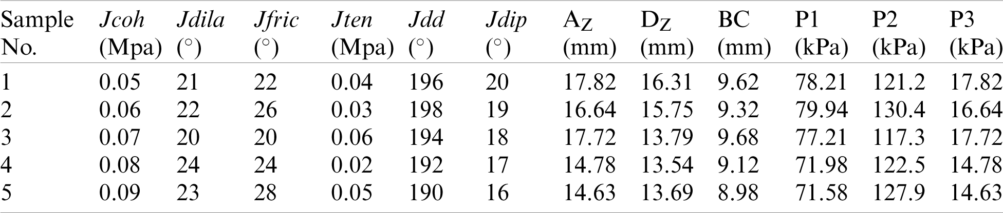
Table 2: The orthogonal parameters schemes and calculated displacements and stress

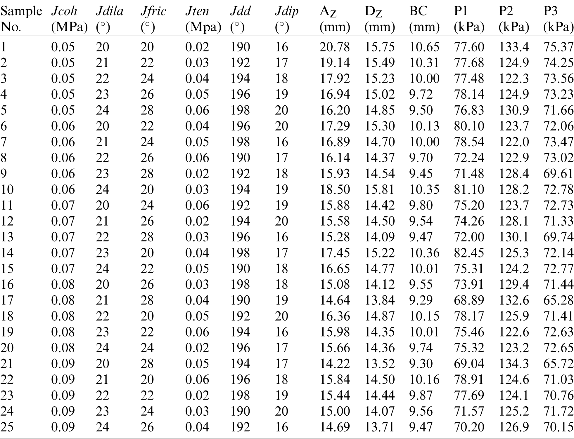
Table 3: The uniformly parameters schemes and calculated displacements and stress

4.3 Parameters Identification Results

Using the engineering monitoring data as the control value, the back analysis of the joint parameters was carried out. The CR was set to 0.9, F was set to 0.6, the maximum evolution algebra was 100, and the population sizes (NP) were set to 100. In the monitoring results of the K7 + 630 m sections, AZ was 14.62 mm, DZ was 13.73 mm, BC was 9.22 mm, P1 was 68.76 kPa, P2 was 131.61 kPa, and P3 was 65.24 kPa. The back analysis results are shown in Tab. 4.

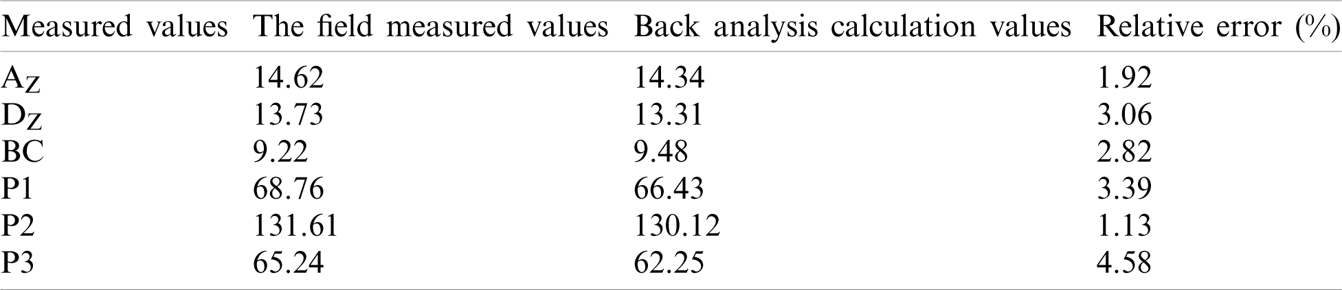
The back analysis joint surface parameters were used to carry out the numerical simulation calculation under the reinforcing measures of the initial lining and pipe-roof of the tunnel, and the displacement variation values of the monitoring points were calculated. The numerical simulation results were compared with the field monitoring data of the K7 + 650 m section, and the comparison results are shown in Tab. 5. As shown in Tab. 5, the maximum relative error of the two methods was 4.58%. Thus, the accuracy of the back analysis results was verified.

Table 4: The back analysis results of joint parameters

Table 5: The results of back analysis and measured data

The fitness values of the GP-DE algorithm population in the first, 3rd, 10th, and 30th generations are presented in Fig. 7, where it can be seen that the distribution of solution vectors in the space gradually decreased and tended to converge with the increase in the evolutionary algebra. The population of the first evolution was relatively dispersed, and the overall fitness value was less than 0.9. The overall fitness value of the 3rd evolution decreased, and it less than 0.4. The overall fitness value of the 10th evolution was also reduced, and it was less than 0.05. The overall fitness value of the 30th evolution was further reduced, and the overall fitness value was less than 1.4 × 10−4.

The changes in the six parameters of the GP-DE algorithm with the number of iterations are presented in Fig. 8. As shown in Fig. 8, at the beginning of the iteration process, the parameters fluctuated and were far away from the optimal solution. With the increase in the iteration step number, the parameters’ values increased, and when the number of iterations reached a value of 30, the parameters tended to the optimal solution and remained stable. Thus, the optimal solution was obtained after 30 iterations, which shows good convergence.

4.4 Surrounding Rock Stability Analysis Based on Identified Parameters

In order to analyze the stability of a jointed surrounding rock and select a rational supporting scheme, the inversion parameters of the jointed rock were used to conduct a numerical simulation to compare the plastic zone of the surrounding rock with different supporting schemes. The four possible reinforcing measures were: initial lining, initial lining + pipe roof, initial lining + pipe roof + pre-stressed anchor, and initial lining + pipe roof + advance grouting anchor. The plastic zones of the tunnel under different reinforcing measures are shown in Fig. 9, where it can be seen that the distributions of the plastic zones around the two tunnels were relatively independent, and the mutual influences of the two tunnels were small. The tunnel construction had a great influence on the stability of the surrounding rock at the top of the tunnel. For the low-grade surrounding rock, the quality of the surrounding rock was poor. The plastic zone distribution of the surrounding rock was minimal when the scheme of the initial lining + pipe roof + advance grouting anchor was used for construction, which was mainly related to the obvious effect of the grouting on improving the surrounding rock parameters.

Under the condition of surrounding rock with joints, the effect of the pre-stressed bolt was small, which was related to the large deformation in the low-grade surrounding rock and the pre-stress loss. When the surrounding rock was grouted, the effect of reinforcement was obviously improved. Therefore, for the reinforcement of a rock wall of a tunnel with a small spacing, it is preferred to grout the surrounding rock to improve the surrounding rock conditions and parameters. Therefore, the scheme of the initial lining + pipe roof + advance grouting anchor is suggested.

5  Discussion

5.1 The Prediction Accuracy of GP Model

The local correlation coefficient σf and noise standard deviation σn denote important hyper-parameters of the GP model. According to the results obtained for the afore-mentioned learning samples and forecast test samples, the hyper-parameters affected the prediction accuracy of the GP model in the logarithmic coordinate system, as shown in Fig. 10. The variations in σf and σn affected the prediction error of the GP, which indicates that proper selection of model parameters is crucial to guarantee the prediction performance. As shown in Fig. 10, at lnσf below −2, the forecast relative error was approximately 12.52%. The mean forecast relative error decreased with the increase in lnσf. When lnσf=5.42 and lnσn=-4.83, the prediction relative error reduced to 2.08%. The variations in the local correlation coefficient σf and noise standard deviation σn affected the GP model prediction error, which shows that it is necessary to select proper parameters to guarantee the prediction performance of the GP. Therefore, the DE algorithm can avoid the random selection of the GP parameters.

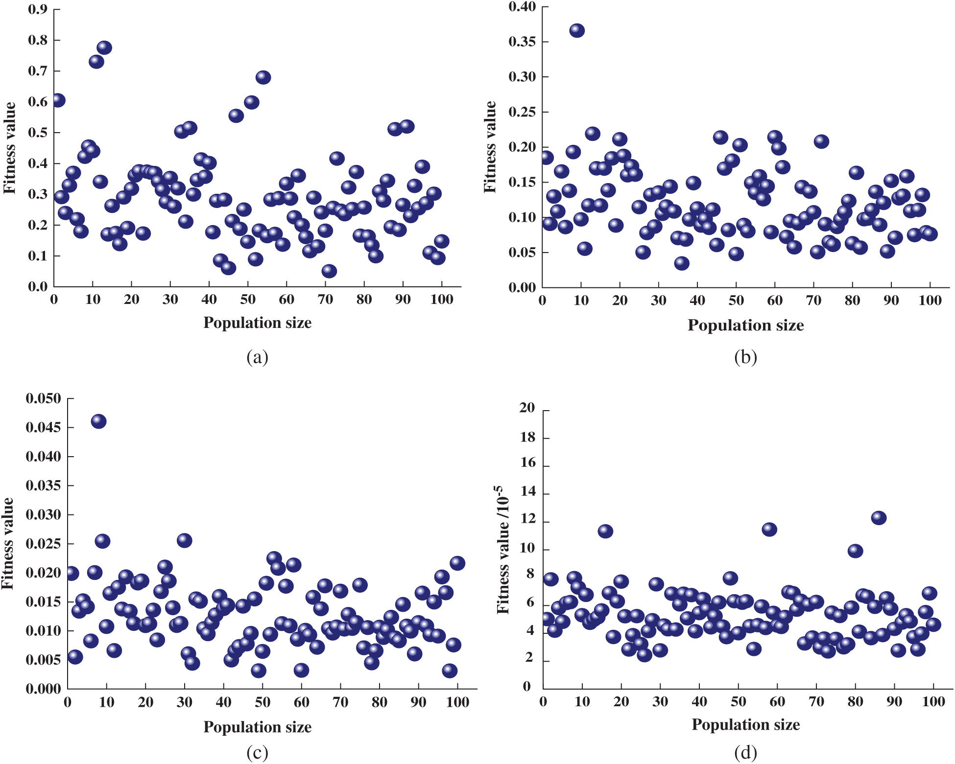
Figure 7: Fitness values with different evolution (a) 1st evolution (b) 3rd evolution (c) 10th evolution (d) 30th evolution

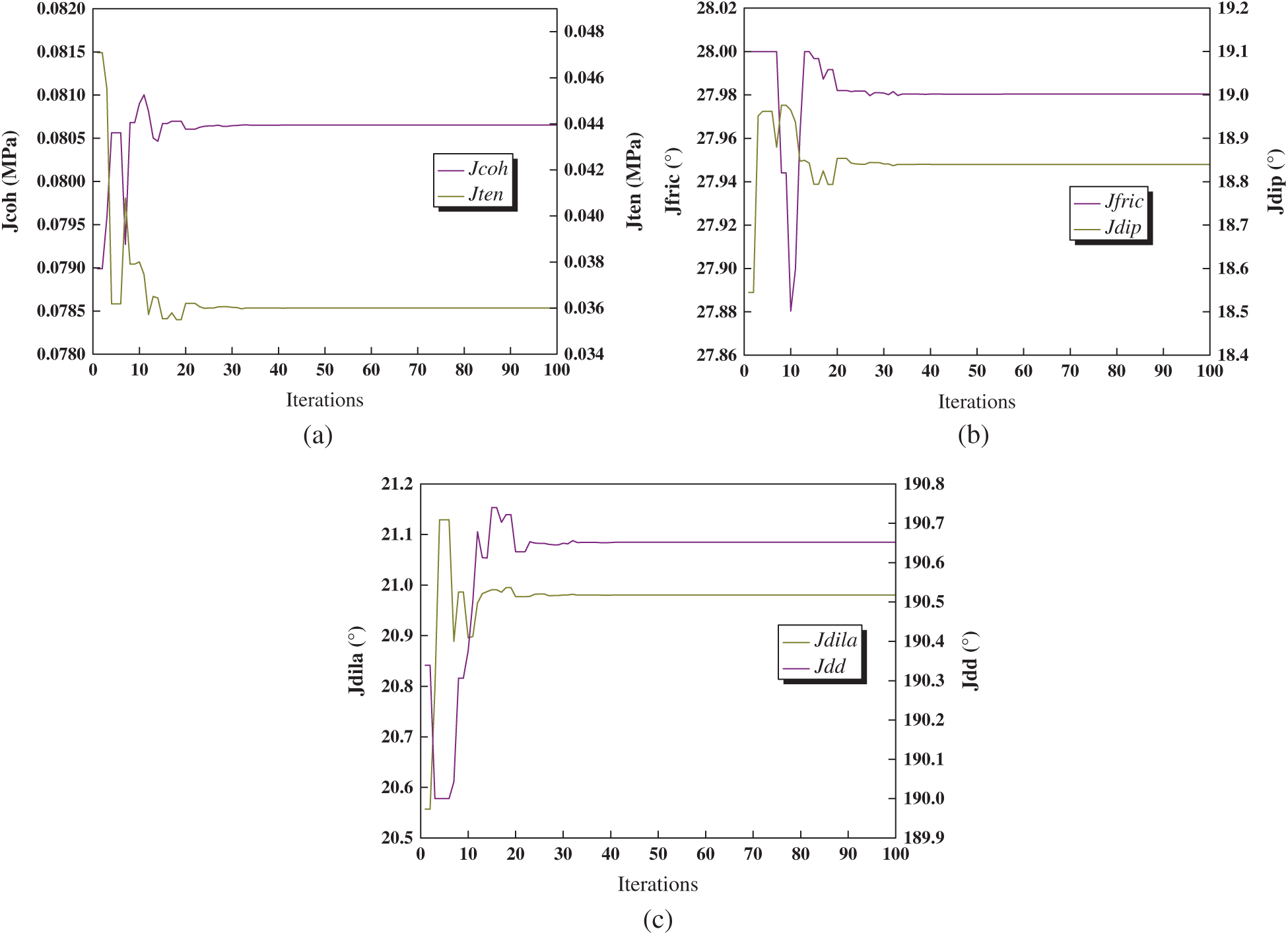
Figure 8: Variation of the parameters (a) Variation of jcoh and jten (b) Variation of jfric and jdip (c) Variation of jdila and jdd

Figure 9: The plastic zone of the tunnel under different reinforcing measures. (a) Initial lining (b) initial lining and pipe-roof (c) initial lining, pipe-roof and pre-stressed bolt (d) initial lining, pipe-roof and advanced grouting bolt

The GP-DE model was compared with the general GP and ANN models, and comparison results are given in Tab. 6. As shown in Tab. 6, among all of the models, the DE-GP algorithm had the highest prediction accuracy of arch settlement and horizontal convergence, while the prediction capabilities of the general GP and ANN algorithm were similar. Compared with the general GP and ANN models, the prediction accuracy of the DE-GP model was greatly improved, and the prediction results were close to the actual displacement calculation results.

5.2 Influence of Differential Evolution Parameters on Optimization Results

In the GP-DE algorithm, the control of the DE algorithm is relatively complex, involving many influencing factors, and it plays a decisive role in the GP-DE algorithm. The back analysis of the joint parameters in the construction site was conducted to discuss the DE algorithm from the two aspects, the control parameters, and different difference strategies.

In the DE, the variation factor F, crossover factor CR, population scale NP, and different difference strategy perhaps have an effect on the convergence speed. In the analysis, the values of variation factor F and crossover factor CR were fixed, and the convergence values of different F and CR values in the iterative process of the algorithm were selected to obtain a comparison curve to analyze their influence on the search process. The iterative convergence curves under different F and CR values are shown in Fig. 11.

For the DE/Best/1 difference strategy and NP = 100, and F = 0.7 and CR between 0.5 and 0.9, the iterative process was stable, and the convergence effect was good. However, there was a difference in the convergence speed. When CR = 0.9, the number of iterative steps reaching the convergence was small. Next, CR was set to 0.9 and F was changed between 0.5 and 0.9. When F = 0.6, the convergence speed was relatively fast. The results show that appropriate initial values of the model parameters can improve convergence speed. Based on the obtained results, CR = 0.9 and F = 0.6 are recommended.

When the DE/Best/1 difference strategy was used, and CR = 0.9 and F = 0.6, and when NP changed from 10 to 200, the iterative convergence curves corresponding to different population sizes were as shown in Fig. 12. As displayed in Fig. 12, with the increase in the population size, the precision of parameter optimization was improved, but the convergence efficiency was reduced. When the population size reached a value of 100, the number of the population continued to increase, and the precision of parameter optimization no longer changed significantly.

Figure 10: The forecast relative error changing according to σf and σn

Table 6: The comparison between the predicted results and the calculated results

In the DE algorithm, different difference strategies can be used to achieve mutation operation, as given in Eq. (20). Selecting F = 0.6, CR = 0.9, and NP = 100, these strategies were compared. As shown in Fig. 13, the convergence efficiency and optimization accuracy of different differential strategies varied in the calculation process. Compared with the other strategies, the DE/Best/1 had a faster convergence speed and higher optimization accuracy in the calculation process.

{DE/rand/1:vi,g=xr1,g+F(xr2,g-xr3,g)DE/best/1:vi,g=xbest,g+F(xr2,g-xr3,g)DE/rand/2:vi,g=xr1,g+F(xr2,g-xr3,g+xr4,g-xr5,g)DE/best/2:vi,g=xbest,g+F(xr1,g-xr2,g+xr3,g-xr4,g)DE/rand-to-best/2:vi,g=xr1,g+F(xbest,g-xr2,g+xr3,g-xr4,g),(20)

Figure 11: Iteration curve with change of CR and F

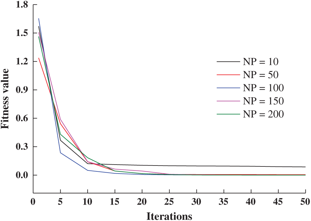
Figure 12: Iteration curve of different population

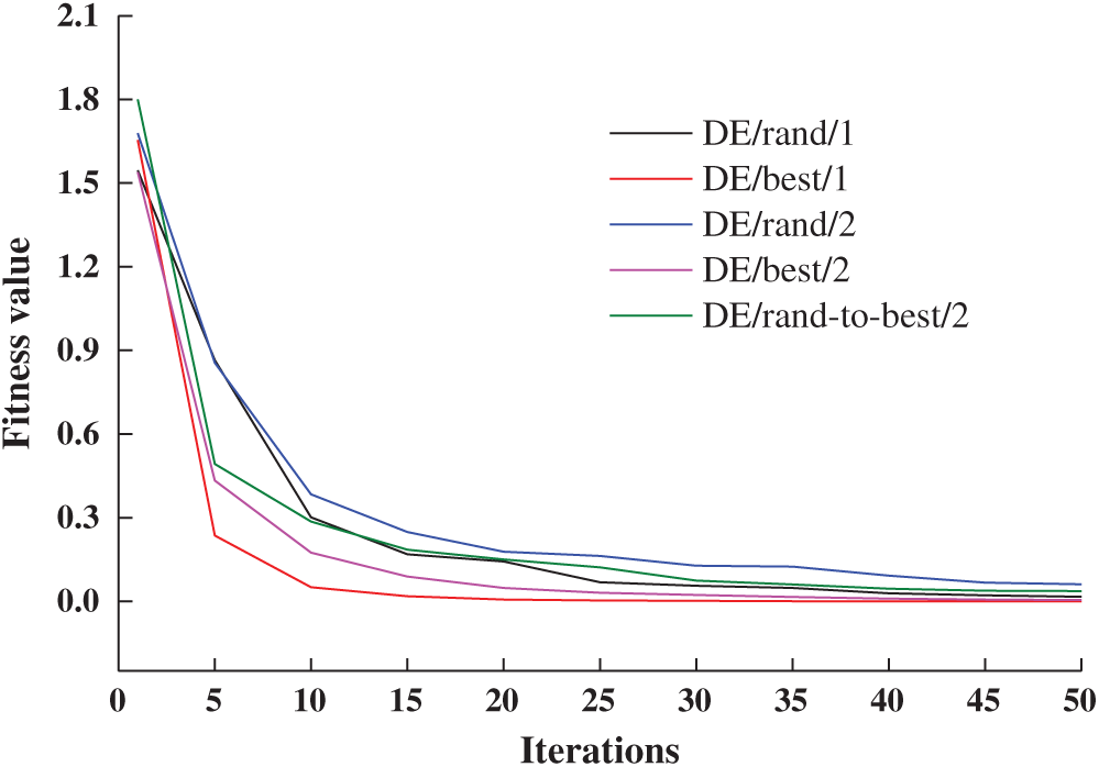
Figure 13: Different differential strategies

6  Conclusions

Aimed at solving the problems of jointed rock parameters identification based on the ubiquitous-joint model and 3D numerical model, the paper proposed a hybrid GP-DE algorithm.

The main contributions of this work can be summarized as follows:

1. In this paper, an orthogonal design, GP, DE, and ubiquitous-joint model are combined to develop a hybrid method for the joint parameters identification of surrounding rock of a tunnel. The proposed method makes full use of the advantages of GP and DE, improves the computing speed, and avoids the problem of result limitation to the local optimal solution. Since hyper-parameters of the GP affect its forecast precision, the DE is used to optimize the GP parameters. Compared with the general GP and ANN models, the proposed GP-DE model has a smaller forecast error.

2. The proposed method is verified by the experiment with a real tunnel, namely, the proposed method is used to invert and analyze the parameters of a joint rock surface in the Dadongshan tunnel project. The results of the back analysis are compared with the field monitored values. The relative error of 4.58% is obtained, which can be considered as a good result. The calculation results show that the proposed method has fast calculation speed, good convergence, and high precision, which can meet the engineering requirements. The variations in the DE parameters have an effect on the convergence speed. Through the calculation and analysis, it has been found that the recommended parameters’ values are CR = 0.9, F = 0.6, and NP = 100, and the difference strategy DE/Best/1 should be used.

3. The identified jointed parameters are considered in the tunnel construction scheme selection and surrounding rock stability analysis. The results show that under the condition of surrounding rock with joints, it is preferred to grout the surrounding rock and rock wall to improve the surrounding rock conditions and parameters. The scheme of the initial lining + pipe roof + advance grouting anchor is suggested.

The results and conclusions presented in this work have guiding significance for tunnel engineering. The paper provides an effective means for the tunnel information construction and feedback analysis with the jointed surrounding rock. However, in the calculation process, different covariance functions need to be selected according to different learning samples.

According to the above discussion, and on the basis of fully grasping the characteristics of various covariance functions, a combined covariance function can be used to improve the accuracy and practicability of the model.

Funding Statement: This work was supported by the National Natural Science Foundation of China (Nos. 51678101, 52078093), Liaoning Revitalization Talents Program (No. XLYC1905015).

Conflicts of Interest: The authors declare that they have no conflicts of interest to report regarding the present study.

References

 1.  Gao, W. (2020). Comparison study on nature-inspired optimization algorithms for optimization back analysis of underground engineering. Engineering with Computers, 34(1), 39. DOI 10.1007/s00366-019-00918-7. [Google Scholar] [CrossRef]

 2.  Kavanagh, K. T., Clough, R. W. (1971). Finite element applications in the characterization of elastic solids. International Journal of Solids and Structures, 7(1), 11–23. DOI 10.1016/0020-7683(71)90015-1. [Google Scholar] [CrossRef]

 3.  Kirstern, H. (1976). Determination of rock mass elastic moduli by back analysis of deformation measurement. Proceedings of Symposium on Exploration for Rock Engineering. Johannesburg. [Google Scholar]

 4.  Oreste, P. (2005). Back-analysis techniques for the improvement of the understanding of rock in underground constructions. Tunnelling and Underground Space Technology, 20(1), 7–21. DOI 10.1016/j.tust.2004.04.002. [Google Scholar] [CrossRef]

 5.  Gioda, G., Maier, G. (1980). Direct search solution of an inverse problem in elastoplasticity: Identification of cohesion, friction angle and in situ stress by pressure tunnel tests. International Journal for Numerical Methods in Engineering, 15(12), 1823–1848. DOI 10.1002/nme.1620151207. [Google Scholar] [CrossRef]

 6.  Yang, C., Wu, Y., Hon, T. (2010). A no-tension elastic-plastic model and optimized back-analysis technique for modeling nonlinear mechanical behavior of rock mass in tunneling. Tunnelling and Underground Space Technology, 25(3), 279–289. DOI 10.1016/j.tust.2010.01.001. [Google Scholar] [CrossRef]

 7.  Gao, X., Yan, E., Yeh, T., Yin, X. M., Cai, J. S. (2020). Back analysis of displacements for estimating spatial distribution of viscoelastic properties around an unlined rock cavern. Computers and Geotechnics, 126(4), 103724. DOI 10.1016/j.compgeo.2020.103724. [Google Scholar] [CrossRef]

 8.  Vardakos, S. S., Gutierrez, M. S., Barton, N. R. (2007). Back-analysis of Shimizu tunnel no. 3 by distinct element modeling. Tunnelling and Underground Space Technology, 22(4), 401–413. DOI 10.1016/j.tust.2006.10.001. [Google Scholar] [CrossRef]

 9.  Das, A. J., Mandal, P. K., Bhattacharjee, R., Tiwari, S., Kushwaha, A. et al. (2017). Evaluation of stability of underground workings for exploitation of an inclined coal seam by the ubiquitous joint model. International Journal of Rock Mechanics and Minning Sciences, 93, 101–114. DOI 10.1016/j.ijrmms.2017.01.012. [Google Scholar] [CrossRef]

10. Das, A. J., Mandal, P. K., Paul, P. S. (2019). Assessment of the strength of inclined coal pillars through numerical modelling based on the ubiquitous joint model. Rock Mechanics and Rock Engineering, 52(10), 3691–3717. DOI 10.1007/s00603-019-01826-4. [Google Scholar] [CrossRef]

11. Ismael, M., Konietzky, H. (2019). Constitutive model for inherent anisotropic rocks: Ubiquitous joint model based on the Hoek–Brown failure criterion. Computers and Geotechnics, 105(2), 99–109. DOI 10.1016/j.compgeo.2018.09.016. [Google Scholar] [CrossRef]

12. Tang, Y., Kung, G. (2009). Application of nonlinear optimization technique to back analyses of deep excavation. Computers and Geotechnics, 36(1–2), 276–290. DOI 10.1016/j.compgeo.2008.02.004. [Google Scholar] [CrossRef]

13. An, J. S., Song, K. I. (2018). Back analysis of an operating subsea tunnel considering the degradation of ground and concrete lining. Marine Georesources & Geotechnology, 37(4), 517–523. DOI 10.1080/1064119X.2018.1427817. [Google Scholar] [CrossRef]

14. Park, H. I., Park, B., Kim, Y. T., Hwang, D. J. (2009). Settlement prediction in a vertical drainage-installed soft clay deposit using the genetic algorithm (GA) back-analysis. Marine Georesources & Geotechnology, 27(1), 17–33. DOI 10.1080/10641190802620198. [Google Scholar] [CrossRef]

15. Moreira, N., Miranda, T., Pinheiro, M., Fernandes, P., Dias, D. et al. (2013). Back analysis of geomechanical parameters in underground works using an Evolution Strategy algorithm. Tunnelling and Underground Space Technology, 33(2), 143–158. DOI 10.1016/j.tust.2012.08.011. [Google Scholar] [CrossRef]

16. Jiang, A. N., Wang, S., Tang, S. (2011). Feedback analysis of tunnel construction using a hybrid arithmetic based on support vector machine and particle swarm optimisation. Automation in Construction, 20(4), 482–489. DOI 10.1016/j.autcon.2010.11.016. [Google Scholar] [CrossRef]

17. Zhang, Y., Su, G., Liu, B. C., Li, T. (2020). A novel displacement back analysis method considering the displacement loss for underground rock mass engineering. Tunnelling and Underground Space Technology, 95, 103141. DOI 10.1016/j.tust.2019.103141. [Google Scholar] [CrossRef]

18. Goh, A., Zhang, Y., Zhang, R., Zhang, W., Xiao, Y. (2017). Evaluating stability of underground entry-type excavations using multivariate adaptive regression splines and logistic regression. Tunnelling and Underground Space Technology, 70(10), 148–154. DOI 10.1016/j.tust.2017.07.013. [Google Scholar] [CrossRef]

19. Lü, Q., Chan, C., Low, B. K. (2012). Probabilistic evaluation of ground-support interaction for deep rock excavation using artificial neural network and uniform design. Tunnelling and Underground Space Technology, 32(4), 1–18. DOI 10.1016/j.tust.2012.04.014. [Google Scholar] [CrossRef]

20. Gao, W., Chen, D., Dai, S., Wang, X. (2018). Back analysis for mechanical parameters of surrounding rock for underground roadways based on new neural network. Engineering with Computers, 34(1), 25–36. DOI 10.1007/s00366-017-0518-x. [Google Scholar] [CrossRef]

21. Zhuang, D., Ma, K., Tang, C., Liang, Z., Wang, K. et al. (2019). Mechanical parameter inversion in tunnel engineering using support vector regression optimized by multi-strategy artificial fish swarm algorithm. Tunnelling and Underground Space Technology, 83(2), 425–436. DOI 10.1016/j.tust.2018.09.027. [Google Scholar] [CrossRef]

22. Su, P., Cai, X., Song, Y., Ma, J., Tan, X. (2020). A hybrid diffractive optical element design algorithm combining particle swarm optimization and a simulated annealing algorithm. Applied Sciences, 10(16), 1–11. DOI 10.3390/app10165485. [Google Scholar] [CrossRef]

23. Miranian, A., Abdollahzade, M. (2013). Developing a local least-squares support vector machines-based neuro-fuzzy model for nonlinear and chaotic time series prediction. IEEE Transactions on Neural Networks and Learning Systems, 24(2), 207–218. DOI 10.1109/TNNLS.2012.2227148. [Google Scholar] [CrossRef]

24. Rasmussen, C. E., Williams, C. (2006). Gaussian processes for machine learning. Adaptive computation and machine learning. Cambridge, Mass: MIT Press. [Google Scholar]

25. Ma, X., Xu, F., Chen, B. (2019). Interpolation of wind pressures using Gaussian process regression. Journal of Wind Engineering and Industrial Aerodynamics, 188(30), 30–42. DOI 10.1016/j.jweia.2019.02.002. [Google Scholar] [CrossRef]

26. Storn, R., Price, K. (1997). Differential evolution–A simple and efficient heuristic for global optimization over continuous spaces. Journal of Global Optimization, 11(4), 341–359. DOI 10.1023/A:1008202821328. [Google Scholar] [CrossRef]

27. An, J. S., Kang, K. N., Choi, J. Y., Sung, W. S., Suy, V. et al. (2020). Tunnel back analysis based on differential evolution using stress and displacement. Advances in Civil Engineering, 2020(5), 1–10. DOI 10.1155/2020/8156573. [Google Scholar] [CrossRef]

28. Yuan, Z. H., Lu, W. (2017). Study on the stress inverse method of mechanical parameters based on coupling of genetic algorithm and finite element. Journal of Railway Science and Engineering, 14(7), 1428–1434. DOI 10.19713/j.cnki.43-1423/u.2017.07.012. [Google Scholar] [CrossRef]

29. Luo, Y., Chen, J., Chen, Y., Diao, P., Qiao, X. (2018). Longitudinal deformation profile of a tunnel in weak rock mass by using the back analysis method. Tunnelling and Underground Space Technology, 71(3), 478–493. DOI 10.1016/j.tust.2017.10.003. [Google Scholar] [CrossRef]

30. Sakurai, S., Takeuchi, K. (1983). Back analysis of measured displacements of tunnels. Rock Mechanics and Rock Engineering, 16(3), 173–180. DOI 10.1007/BF01033278. [Google Scholar] [CrossRef]

31. Lu, R., Wei, W., Shang, K., Jing, X. (2020). Stability analysis of jointed rock slope by strength reduction technique considering ubiquitous joint model. Advances in Civil Engineering, 2020(1), 1–13. DOI 10.1155/2020/8862243. [Google Scholar] [CrossRef]

This work is licensed under a Creative Commons Attribution 4.0 International License, which permits unrestricted use, distribution, and reproduction in any medium, provided the original work is properly cited.