| Computer Modeling in Engineering & Sciences |
DOI: 10.32604/cmes.2021.015894
ARTICLE
A Combined Shape and Topology Optimization Based on Isogeometric Boundary Element Method for 3D Acoustics
CAS Key Laboratory of Mechanical Behavior and Design of Materials, Department of Modern Mechanics, University of Science and Technology of China, Hefei, 230026, China
*Corresponding Author: Haibo Chen. Email: hbchen@ustc.edu.cn
Received: 21 January 2021; Accepted: 18 February 2021
Abstract: A combined shape and topology optimization algorithm based on isogeometric boundary element method for 3D acoustics is developed in this study. The key treatment involves using adjoint variable method in shape sensitivity analysis with respect to non-uniform rational basis splines control points, and in topology sensitivity analysis with respect to the artificial densities of sound absorption material. OpenMP tool in Fortran code is adopted to improve the efficiency of analysis. To consider the features and efficiencies of the two types of optimization methods, this study adopts a combined iteration scheme for the optimization process to investigate the simultaneous change of geometry shape and distribution of material to achieve better noise control. Numerical examples, such as sound barrier, simple tank, and BeTSSi submarine, are performed to validate the advantage of combined optimization in noise reduction, and to demonstrate the potential of the proposed method for engineering problems.
Keywords: Combined shape and topology optimization; isogeometric boundary element method; shape sensitivity analysis; topology sensitivity analysis; adjoint variable method; sound absorption material
Isogeometric analysis (IGA) [1] has been proposed to eliminate the gap between computer-aided design (CAD) and computer-aided engineering (CAE), where non-uniform rational basis splines (NURBS) are widely used to represent geometry and approximate physical field variables, due to its advantages such as accurate description of geometry, high-order continuous fields, and flexible refinement. Compared with the finite element method (FEM) [2], boundary element method (BEM) [3] has exhibited superior performance in problems like exterior acoustics [4] because of its advantages including discretizing in boundary and fitting for infinite domain problems. The fully coupled FEM–BEM algorithm [5] was also proposed for acoustic-structural optimization design [6] to exploit the benefits of the two methods. Besides, various accelerated techniques such as adaptive cross approximation (ACA) [7], fast multipole method (FMM) [8–11], and wideband FMM [4,12,13], have also been adopted to improve BEM’s computational efficiency for large-scale problems. Considering that complex structures are usually described by NURBS patch in CAD software, which means that the geometry model are boundary-represented, the isogeometric boundary element method has also been successfully applied to potential problems [14–17], elastic problem [18–20], and acoustics [21–24]. FEM–BEM coupled analysis method was also combined with IGA in elasticity [25]. As the NURBS control points play a critical role in geometry construction, it is highly flexible to change the structural geometric shape. Refinement operators [1] such as h-refinement, p-refinement, and k-refinement have also been proposed to perfect IGA. Thus, conducting optimization design via IGA BEM is convenient.
The problem of sound emission of structures has attracted much attention in engineering practice. Structures such as sound barriers have also been investigated for their acoustic performance [26,27] in noise control. Baulac et al. [28] performed an optimization design of a sound barrier via BEM. Chen et al. [29] studied the distribution of absorbing material on a noise barrier by optimization design. Zhao et al. [30] applied topology optimization to the distribution of sound absorption material (SAM) that covers the structural surface with FMM BEM. Zhao et al. [31] also investigated the topology optimization of two different materials based on FEM–BEM coupled method. Liu et al. [32] and Chen et al. [33] conducted the sound barrier’s shape optimization by IGA BEM in 2D acoustics. Among these approaches, shape optimization and topology optimization are mainly used for designing structures to change their acoustic performance.
Shape optimization plays a great role in engineering problems to obtain the optimal shape under certain constraints with objectives. In this rational and automatic process, the geometry shape needs to be regenerated in each step, which causes limitation in conventional numerical analysis. In IGA, the structure surface is constructed by NURBS control points with weights and knot vectors; thus, the surface is easy to change by defining the control points as design parameters. Although IGA FEM has been firstly combined with shape optimization in fluid mechanics [34] and electromagnetism [35], IGA BEM is more suitable for the surface shape change in shape optimization, due to NURBS’ and BEM’s features. Shape optimization has also been conducted through IGA BEM in heat conduction [36], wave resistance [37], elasticity [38–40], and acoustics [13,32,41]. In engineering problems, sound structures may be covered with SAM or other materials. Different from design structure surface shape, the topology optimization focuses on finding the best topological distribution of SAM on the surface. Chen et al. [33] firstly conducted the topology optimization of the distribution of SAM on the sound barrier surface by IGA BEM with NURBS. Chen et al. [42] also studied the distribution of SAM via IGA BEM with subdivision surface method for 3D acoustics. Their findings demonstrated the frequency-dependent phenomenon in acoustic optimization design.
The previous works mainly conduct one type of optimization method to improve acoustic performance of structures. The present study focuses on combining the shape and topology optimization together efficiently to ensure better noise control for 3D acoustic problems. For combined optimization, researchers have done many works with the level set method (LSM) to conduct shape and topology update simultaneously by a uniform manner [43–45]. Matsumoto et al. [44] adopted the LSM in the acoustic scatter problem to design the shape and topology of the structure. In this work, the topology optimization we considered is the distribution of SAM on structural surface. The solid isotropic material with penalization (SIMP) [46] method is applied to the initialization of design variables by converting the discrete density values of artificial material into continuous variables and enabling the intermediate density to approach 0 or 1, where 0 means that no material is on the design area. Thus, we select another type of combined optimization, where the shape and topology of structure should be changed by constructing a connection between them. Researchers have applied the deformable simplicial complex (DSC) method to combine shape and topology optimization in elasticity problems [47–49], where the topology design variables were updated first, and then the shape update was implemented subsequently. This process was called total iteration step of the combined optimization. Lin et al. [50] performed shape and topology optimizations through a time-dependent adjoint approach for sensitivity analysis in 2D acoustic metamaterials and phononic crystals, where shape optimization followed the topology optimization subsequently to modify the structural geometries. Jiang et al. [51] compared four iteration schemes by the second kind of combined optimization and successfully applied them to the noise reduction on sound barriers based on IGA BEM in 2D acoustics. In this paper, we mainly expand the best iteration scheme proposed by Jiang et al. [51] to 3D acoustics and applied it to complicated structures, where the NURBS control points coordinates are set as design parameters for shape design, and the artificial densities on NURBS integral elements are selected as the design variables for topology analysis. As both the two types of parameters are related to IGA BEM, a bridge is constructed between the structural shape and the distribution of SAM on the surface, which helps the shape and topology change in each iteration step. Meanwhile, using IGA BEM also avoids mesh regeneration, which improves the efficiency in the optimization process.
To implement combined optimization, the gradient-based optimizer is generally used due to its high efficiency, for example, the method of moving asymptotes (MMA) [52]. This condition leads to the requirement of gradient information, which means additional step, i.e., sensitivity analysis. The present study consists of two parts: shape sensitivity analysis with respect to the control points, and topology sensitivity analysis with respect to the artificial densities. Finite difference method (FDM), direct differentiation method (DDM) [4,12,53], and adjoint variable method (AVM) [30,54,55] are the three main methods for both the two types of sensitivity analysis. The DDM and AVM provide the analytical expression of sensitivity, and the AVM shows higher efficiency for multiple design variables. As the shape design parameters and topology design variables may be large in engineering, AVM is more suitable for ordinary optimization problems to achieve high efficiency. Here, we adopt the AVM for both the two types of sensitivity analysis. Another difficulty in IGA BEM for 3D acoustics is the non-uniqueness problem [56,57], especially for exterior acoustics. The Burton–Miller method [56,58] is adopted to overcome this problem, where Marburg [59] has investigated the influence of different coupling parameters on the analysis result. However, using this method also results in the problem of hyper singular integrals [41]. Thus, the method based on subtraction of singularity technique [41,60] is also adopted to compute the singular integrals to achieve high accuracy. Moreover, to improve the efficiency of analysis conveniently, OpenMP tool in Fortran code is exploited in the matrix computation without changing the formulation of IGA BEM.
The present work is devoted to extending the combined optimization algorithm to 3D acoustics. The rest of this paper is organized as follows. In Section 2, the IGA BEM for 3D acoustics with the impedance boundary conditions are reviewed. Section 3 discusses the sensitivity analysis via AVM with respect to the NURBS control points and the artificial densities of SAM, respectively. Section 4 describes the three optimization procedure: shape optimization, topology optimization, and combined optimization. Section 5 introduces several numerical examples to validate the proposed approach. Finally, Section 6 provides the conclusions of this work.
2 Isogeometric BEM for 3D Acoustics
In IGA, we can define the knot vector
For pg > 1, we have the following basis functions:
Then, a B-spline curve’s formulation can be described by
where
For B-spline surface, we need two knot vectors
By introducing a weight
Similarly, the NURBS surface formulation can be described as follows:
where the number of control points is represented by
2.2 Isogeometric BEM for Acoustics
Considering a domain
where p denotes the sound pressure,
For boundary element method, by applying Green’s second theorem and letting point
where
The Green’s function for 3D acoustics is given as follows [41]:
where
In this study, we consider the impedance boundary condition
where
In IGA BEM, the NURBS interpolations are applied to both the geometry and physical fields. In this study, we adopt different NURBS interpolation formulations to suit physical analysis, which means that the physical field is separated from the geometry. The knot vectors of the physical space can be represented as
where pl and ql denote the sound pressure and flux coefficients associated with the l-th physical control point, respectively; Nd is the total number of physical control points; and
The location of collocation points in parametric space can be obtained by the Greville abscissa as follows:
where pd1 and pd2 denote the orders of basis function of each dimension, respectively; nd and md are the number of collocation parameters in each dimension, and
Similarly, after discretizing the boundary into
where
When the parameter
By adopting the Burton–Miller formulation [58] with coefficient
where
After Eq. (21) is solved, the sound pressure of points lying in the domain can be obtained by
where the computations of matrices
3 Sensitivity Analysis through IGA BEM
Sensitivity analysis can obtain the derivatives of objection function with respect to different kinds of design variables. Thus, this type of analysis plays a critical role in the optimization process. The shape sensitivity and topology sensitivity analyses are presented in this section.
3.1 Shape Sensitivity Analysis
Control points usually control the configuration of structure surface in IGA, which means that they can be naturally set as the design parameters in shape optimization. In this study, we set certain control points of the NURBS surface as design parameters to change the shape, and the AVM proposed by Zheng et al. [54] is adopted for shape sensitivity analysis.
In DDM, Eqs. (8) and (9) can be differentiated with respect to the design parameter
where the sensitivities of the kernel function are presented as
The sensitivity interpolation by NURBS basis functions are presented as
where
Similarly, using the same discretization as in Eq. (19), we can express Eqs. (23) and (24) as
Subsequently, still based on the Burton–Miller formulation, Eqs. (32) and (33) can be combined and expressed by matrix form as
where matrices
For sensitivity analysis via DDM, after Eq. (34) is solved, the source point
where the computation of
However, some engineering problems may require more design parameters to guarantee the complexity of the structure, and the objective function in the optimization process may be merely related to physical values at field points. Thus, the AVM is adopted for ordinary optimization design. In accordance with Eqs. (34) and (35), the formulation can be rewritten as
where the calculation of
and thus, the value of adjoint matrix
Finally, by substituting Eq. (38) into Eq. (36), we can calculate the new formulation for the shape sensitivities at field points as follows:
Evidently, the adjoint matrix
3.2 Topology Sensitivity Analysis
In this study, we investigated the topology optimization of the distribution of SAM on structural surface, which is a problem with discrete values of 0 or 1, so that the mathematical computation in sensitivity analysis can be conducted. The SIMP method [46] is adopted to transform the discrete values into continuous values. The artificial density
where
As the artificial density of the material of each element is set as a design variable, the AVM is also implemented for higher efficiency in topology sensitivity analysis. Usually, the objective function is related to the sound pressure of the field points as
where
The derivatives of objective function
where the term u3 does not contain any term about
Combining Eq. (42) with Eq. (43) yields
As both
and by solving Eq. (45), the derivative of objective function can be obtained by
Evidently, both the adjoint operators
4 Combined Shape and Topology Optimization
In this work, we present the combined shape and topology optimization to change the geometric shape and distribution of SAM on structural surface simultaneously. IGA BEM is applied to gradient-based optimization algorithm to construct a bridge between these two types of optimization process. After obtaining the two types of sensitivities in Section 3, we select the method of moving asymptotes (MMA) developed by Svanberg [52] as the optimization solver to update the design variables in each iteration step.
The optimization model of shape optimization can be described as follows:
where the objective function
where
In each iteration step, the design parameters are updated until the objective function
As mentioned in Section 3.2, we change the distribution of SAM to minimize the average SPL of observed points. The optimization model is expressed as
where vse denotes the volume of the e-th NURBS element. Vs0 denotes the volume constraint of the total materials, and we usually set it as half of the surface volume of the structure, which means that the volume fraction should be less than 0.5.
In the topology optimization, we select the same objective function and its sensitivity as those in shape optimization, where the values of
Then, we can compute
According to Chen et al. [33], both shape optimization and topology optimization exhibit good acoustic performance. For single shape optimization or topology optimization, the main process shown in Figs. 1a and 1b mainly includes the input of the NURBS model, initialization of the optimization model, acoustic analysis based on IGA BEM, shape or topology sensitivity analysis, and optimization solver through MMA to update the design parameters/variables.
In this study, the target is to combine the geometry shape change and distribution of SAM simultaneously to achieve better acoustic performance than the single type of optimization. Thus, the key is to select a suitable iteration scheme to combine these two types of optimization process. Considering the computational efficiency and their features in the optimization process, the presented scheme is shown in Fig. 1c, where each outer iteration step includes an inner iteration process that consists of a converged topology optimization and a one-step shape optimization. Although we have used the SIMP method, some elements may still exhibit intermediate densities between 0 and 1, which are the so-called gray elements. Here, the density operator based on a smoothed Heaviside function is adopted to eliminate these elements, and the detailed formulation was discussed by Zhao et al. [30].
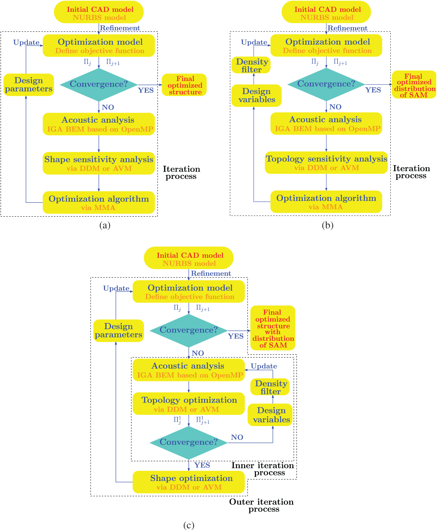
Figure 1: Flow chart of three optimization processes based on IGA BEM (a) Shape optimization process (b) Topology optimization process (c) Combined optimization process
Several numerical examples are presented to validate the applicability of the proposed approach and show its potential in engineering problems. Here, all the examples are exterior acoustic problems, and the parameter
A scattering sphere model is considered to verify the shape sensitivity analysis and topology sensitivity analysis of the present approach. The sphere center is located at point (0, 0, 0) with a radius
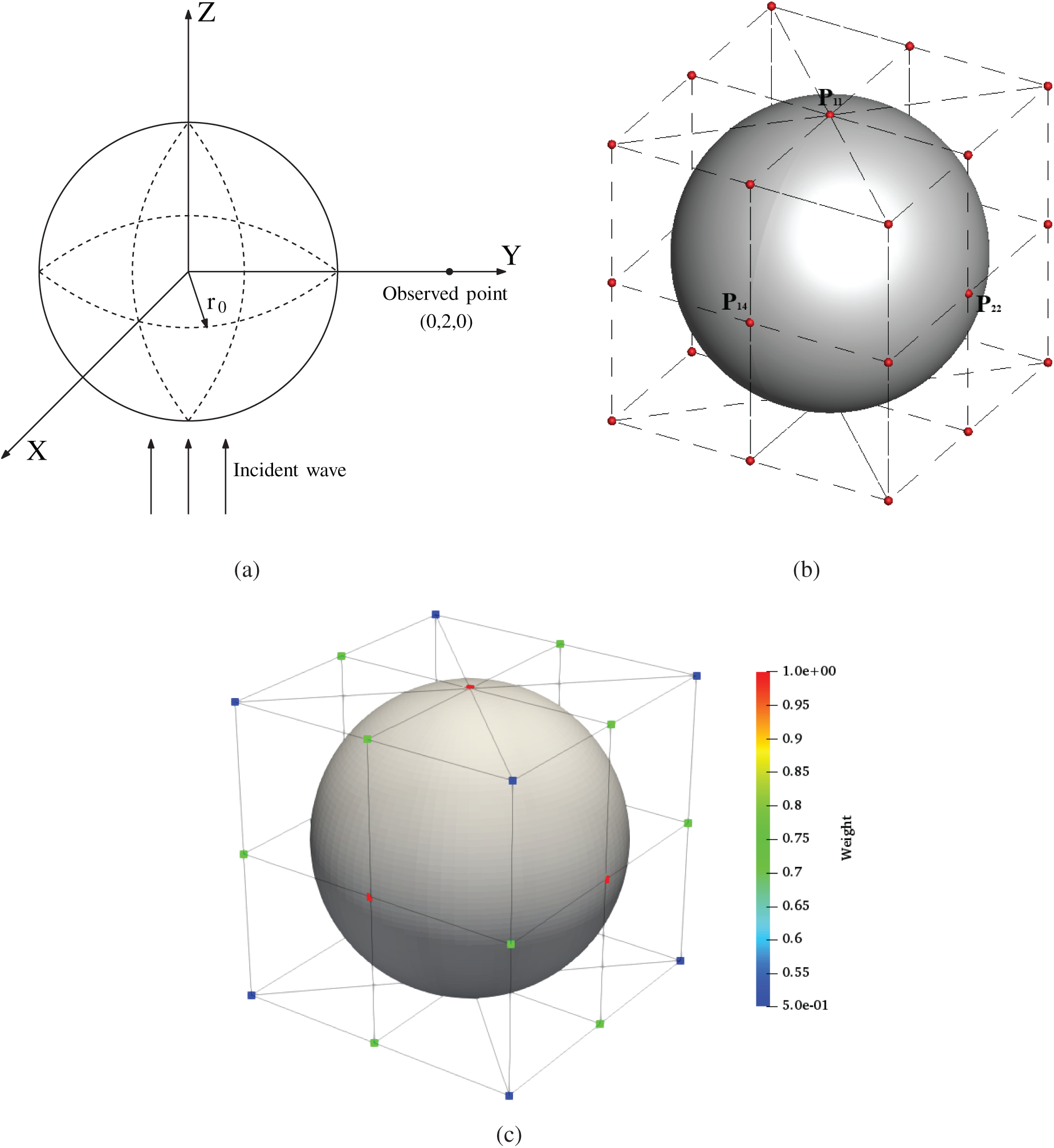
Figure 2: Scattering sphere (a) Physical model (b) NURBS model with control points (c) Weights for control points
Fig. 3 shows the computation time of IGA BEM on acoustic analysis accelerated by OpenMP tool, where the more threads used in computation, the less time is needed. As the figure shows, the efficiency of OpenMP tool using 56 threads can be 20 times faster than the ordinary code. Moreover, compared with the FMM [32], adopting OpenMP tool only needs to change a few for the code, which becomes more convenient for the analysis.
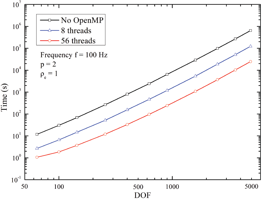
Figure 3: Computing times of IGA BEM accelerated via OpenMP tool on acoustic analysis
For the computation of sound sensitivities with respect to shape parameters, the y-coordinate of the control point
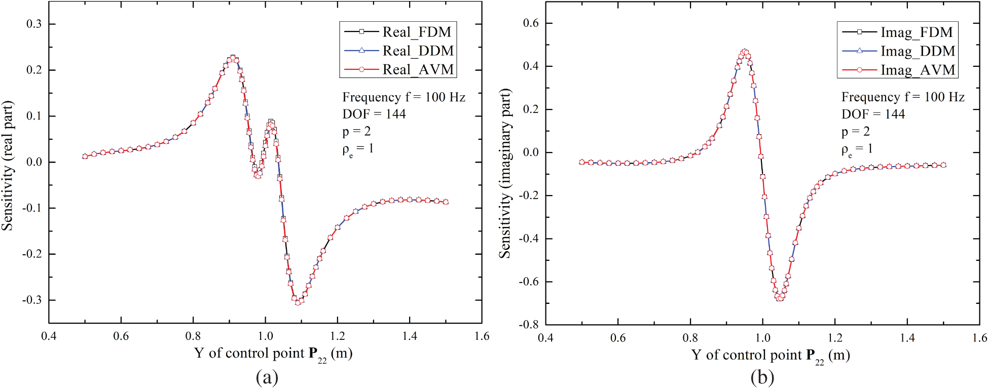
Figure 4: Sound pressure sensitivities at point (0, 2, 0) with respect to y-coordinate of control point
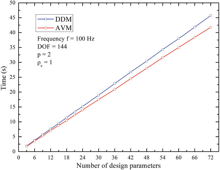
Figure 5: Computing times of DDM and AVM in obtaining sensitivities of the observed point
The verification of topology sensitivity analysis is also shown in Fig. 6, where we set the objective function as the SPL at the observed point. The result of AVM is also compared with those of DDM and FDM. As the figure shows, the three methods provide the same results in sensitivities of the objective function, which validates the correctness of the analytical algorithms, i.e., DDM and AVM. Fig. 7 reveals the efficiency of the DDM and AVM in topology sensitivity analysis. When the number of design variables is less than 256, the DDM takes less time than the AVM, while the AVM shows higher efficiency when the number of design variables is larger than 256. Furthermore, the results of efficiency in Figs. 5 and 7 also demonstrate that topology sensitivity analysis usually takes less time than shape sensitivity analysis, even if we set more design variables for topology analysis. The reason is that the computation of shape sensitivity in matrices
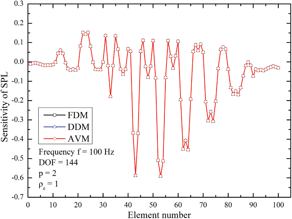
Figure 6: Sensitivities of SPL at point (0, 2, 0) with respect to artificial density
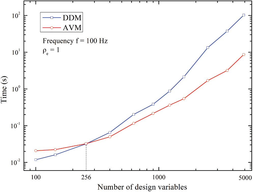
Figure 7: Computing times of topology sensitivity evaluation via DDM and AVM
Although sound barriers have been simplified as 2D problems for optimization design by using the IGA BEM in the work of Liu et al. [32] and Chen et al. [33], we conduct a more practical 3D model for
where
As shown in Fig. 8, a mono-pole source is located at point (0, 1, 1), and the initial state of the barrier is that all the surfaces are covered with SAM. The NURBS model is discretized by 1156 integral elements. After the IGA discretization, the maximum element size is about
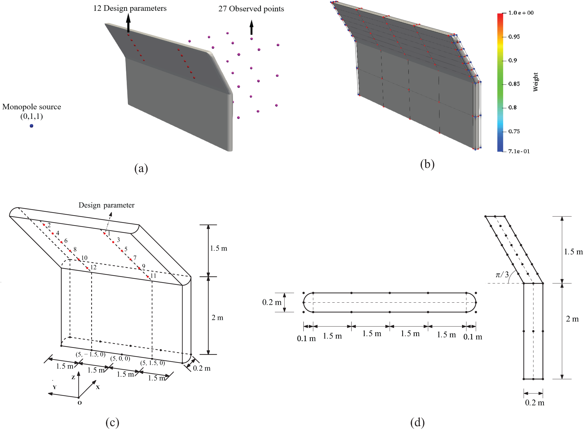
Figure 8: Initial sound barrier model (a) Physical model (b) NURBS model (c) Size of sound barrier (d) Cross section
Table 1: Design parameters in sound barrier model for shape optimization
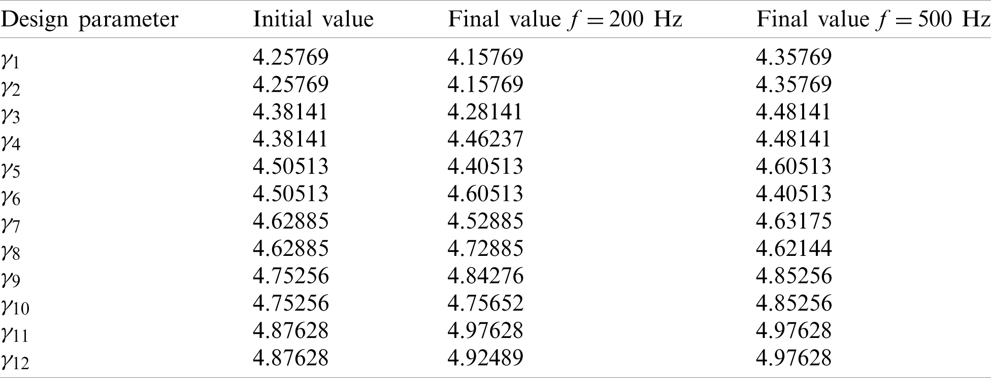
Fig. 9 shows the iteration histories of the objective function by using the three optimization methods. Compared with the other two methods, the shape optimization is only reduced slightly for the average SPL at the lower frequency of
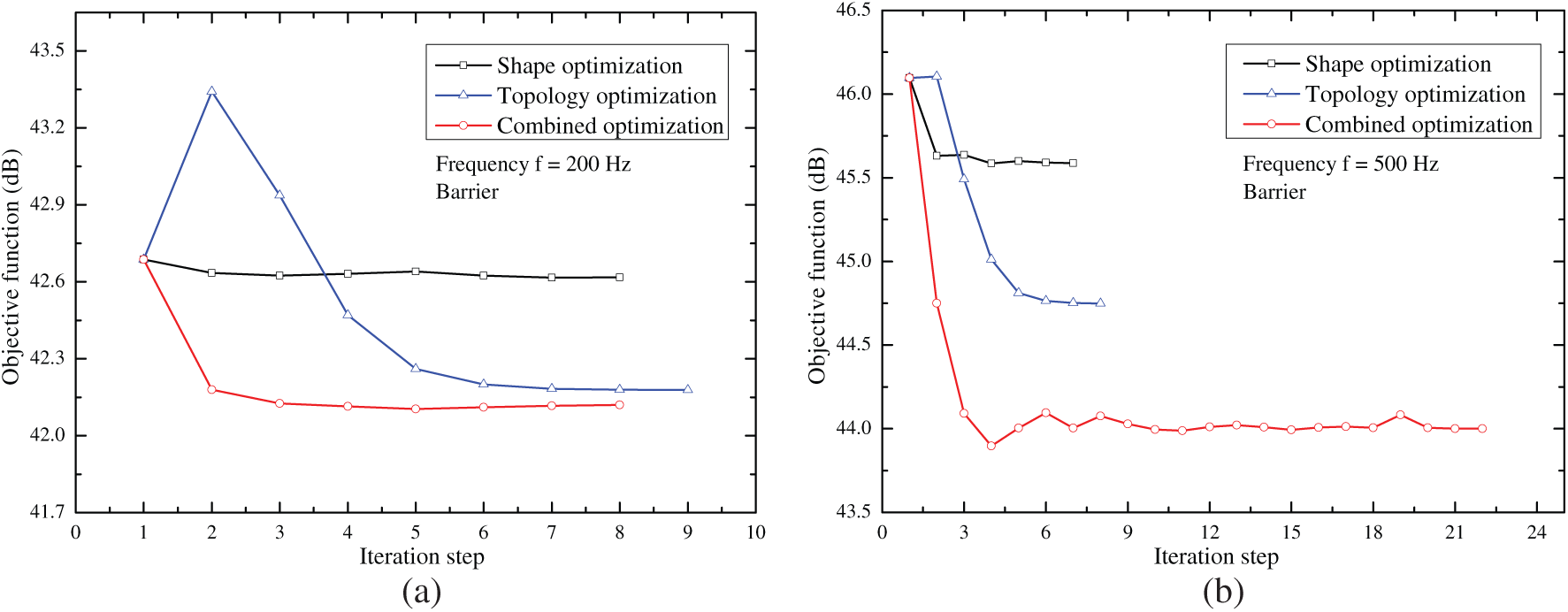
Figure 9: Iteration histories of sound barrier’s objective function by using three optimization methods (a) Frequency
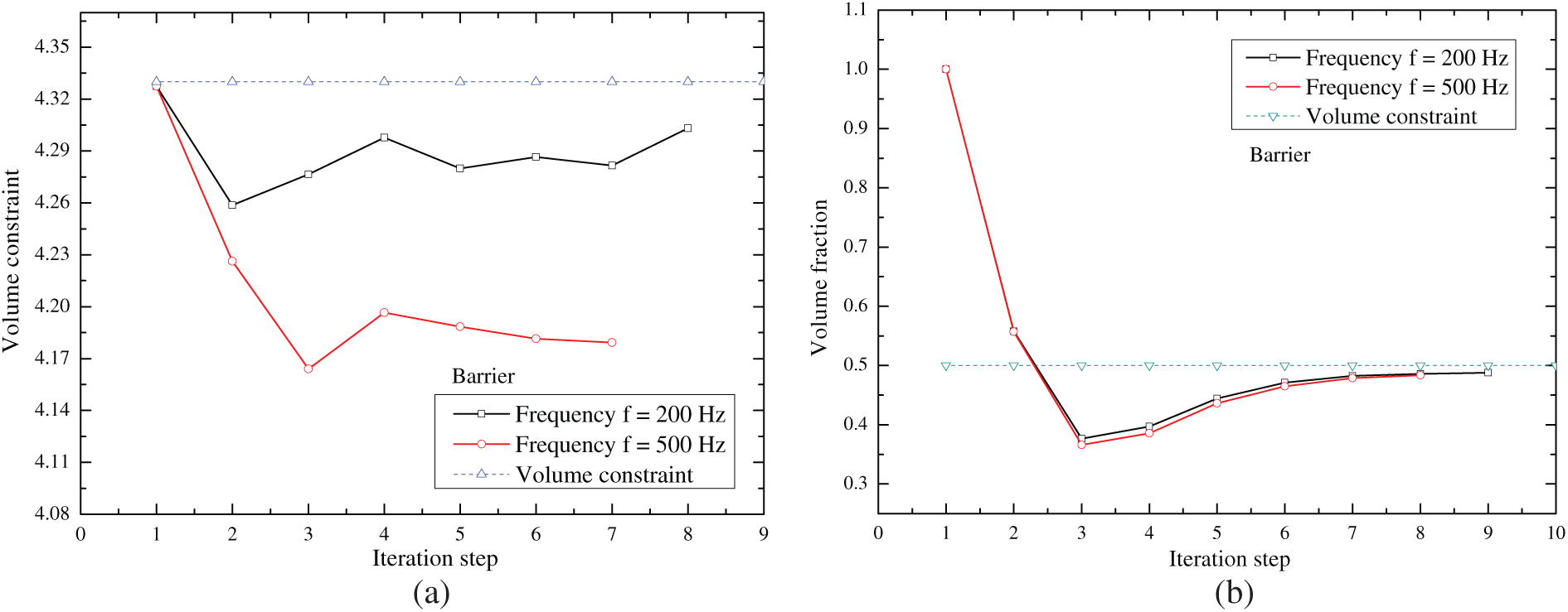
Figure 10: Iteration histories of sound barrier’s volume constraint for shape optimization and topology optimization (a) Shape optimization (b) Topology optimization
Figs. 11 and 12 show the optimization results of the sound barrier by using the three optimization methods. As Tab. 1 shows, the final optimized shape changes slightly compared with the initial structure in the shape optimization process, which means that the range of shape design parameters may not be large, while a larger range of lower and upper bounds usually offers more values for design parameters to be chosen in each optimization iteration step. For the results of topology optimization, the distribution layout of SAM tends to occupy many smaller areas at a higher frequency of
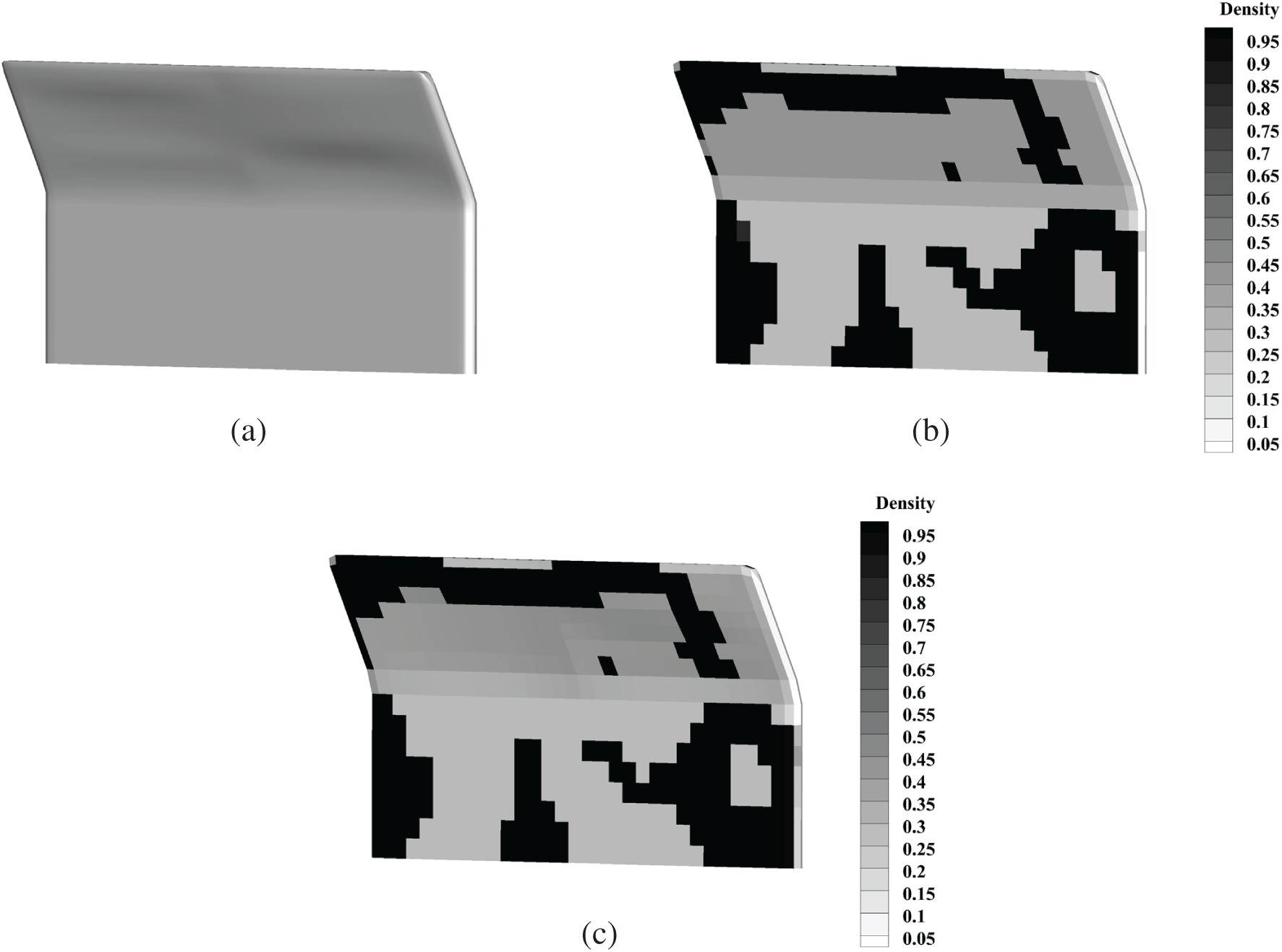
Figure 11: Optimization results of sound barrier by using three optimization methods at frequency
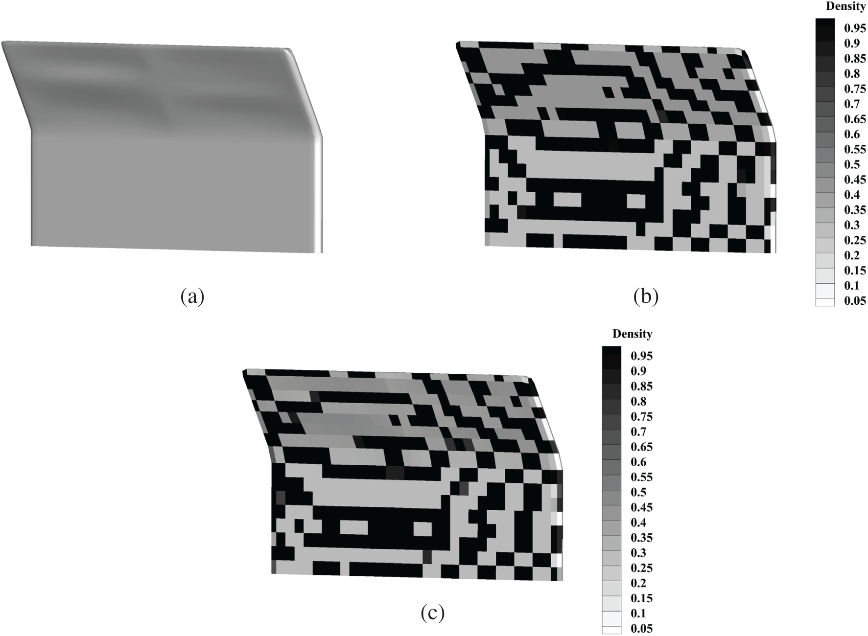
Figure 12: Optimization results of sound barrier by using three optimization methods at frequency
For the topology optimization at a higher frequency of
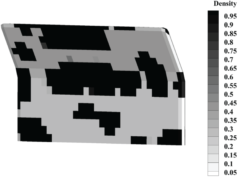
Figure 13: Optimization results of sound barrier with filter radius
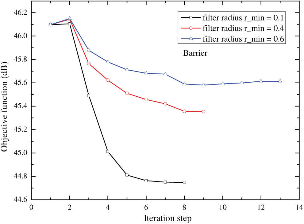
Figure 14: The impact of filter radius on objective function for sound barrier’s topology optimization at frequency
The example of a underwater simple tank presented by Chen et al. [41] is analyzed in this section. Fig. 15 shows the model in physics and geometry. Herein, the wave velocity is
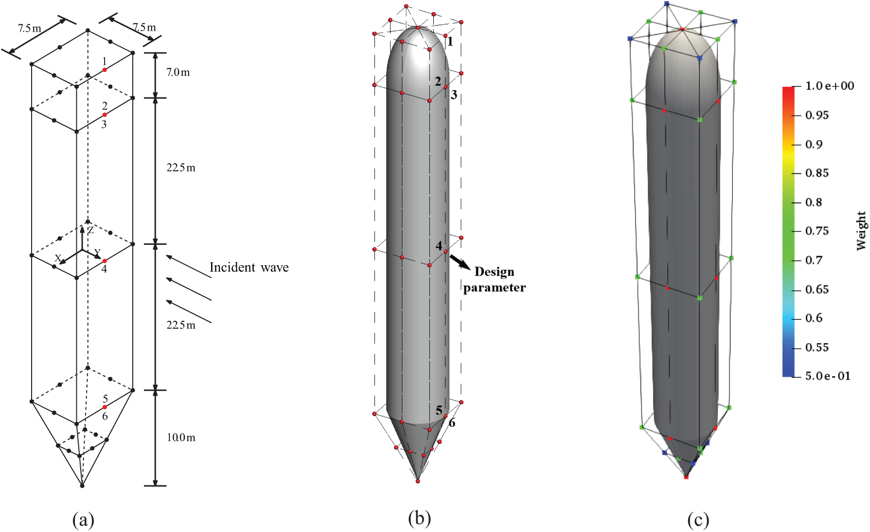
Figure 15: Initial simple tank model (a) Physical model (b) NURBS model with control points (c) Weights for control points
Table 2: Design parameters in simple tank model for shape optimization
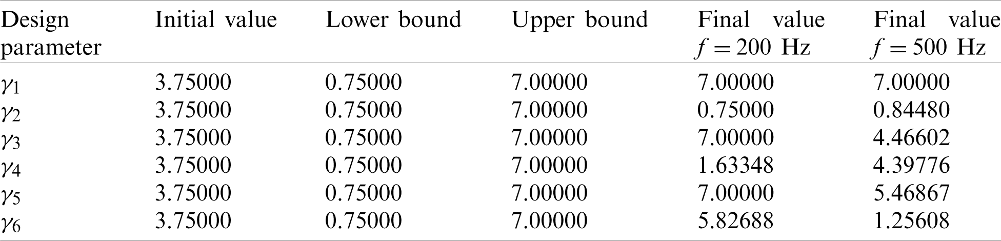
Fig. 16 shows the iteration histories of objective function for the three optimization methods on the simple tank. We have expanded the range of parameters for shape design, as depicted in Tab. 2; thus, this time the shape optimization achieves a good noise reduction, even better than the topology optimization at
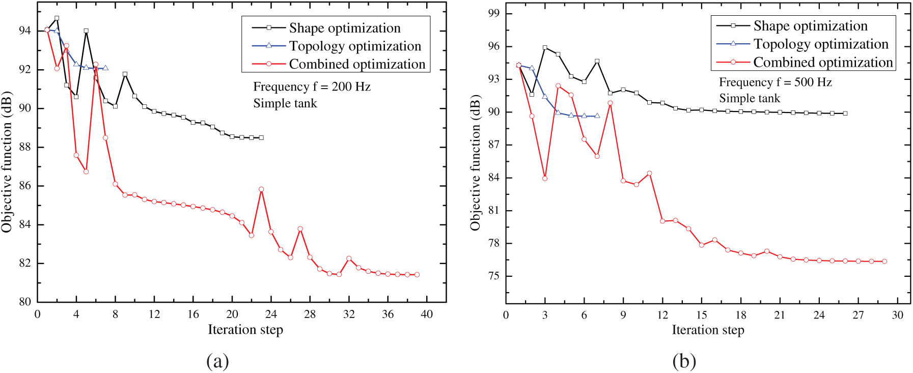
Figure 16: Iteration histories of objective function of simple tank using three optimization methods (a) Frequency
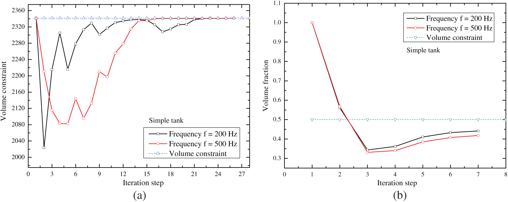
Figure 17: Iteration histories of simple tank’s volume constraint for shape optimization and topology optimization (a) Shape optimization (b) Topology optimization
Figs. 18 and 19 show the optimization results of simple tank by using the three optimization methods. Compared with the initial structure, the optimized shapes have changed obviously after shape optimization and combined optimization. This is mainly due to the expanded side range of the shape design parameters. For topology optimization, the SAM tends to be more spread at higher frequency. However, few gray elements still appear after the optimization, although we have conducted a density filter operator. Finally, the combined optimization also shows a detailed change in shape or distribution of material compared with the single type of optimization. These figures also demonstrate that the phenomenon of frequency dependence for optimized shape and distribution of material is clear.
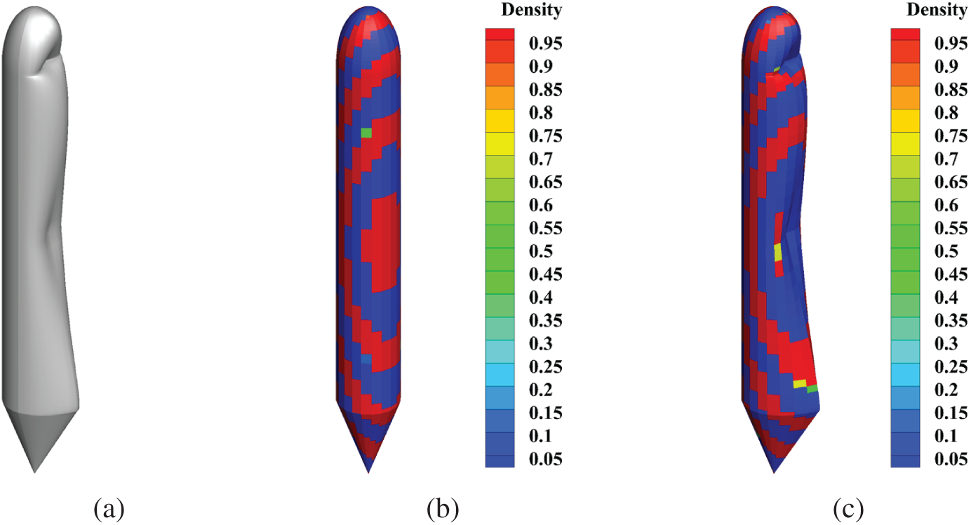
Figure 18: Optimization results of simple tank by using three optimization methods at frequency
Figure 19: Optimization results of simple tank by using three optimization methods at frequency
An obvious checker-board phenomenon is also indicated by Fig. 19b, and thus, we also test the mesh-dependency problem. As exhibited in Fig. 20, the checker-board phenomenon still appears if we only keep the filter radius rmin as a small value
Figure 20: Topology optimization result of simple tank with 6400 NURBS elements and filter radius
Figure 21: Topology optimization result of simple tank with filter radius
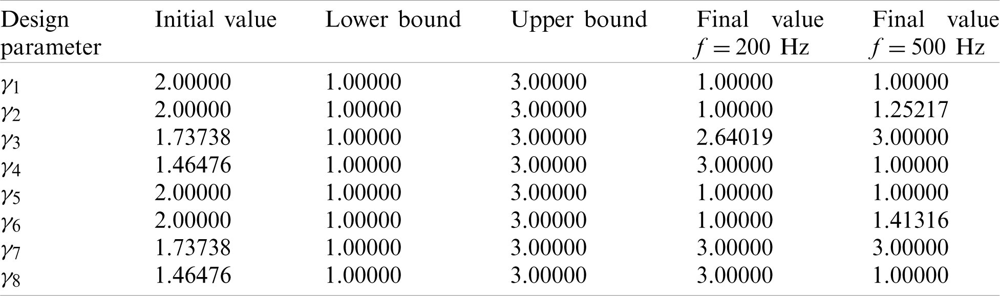
To exhibit the capability of the proposed algorithm in optimization design of complicated geometry, the BeTSSi submarine model described by Venås et al. [22] is considered in this section. Now we adopt a half size scale of this model for analysis. Moreover, we have reconstructed the submarine by NURBS, where the submarine consists of 7 NURBS patches; thus, the optimization based on IGA BEM for 3D acoustics is extended to the problem of multi-patch structures [64]. The discontinuous element method [64,65] is also applied to IGA BEM for 3D acoustics. Figs. 22a and 22b show the submarine’s NURBS model, control points, and weights. Shape design parameters are set as the z-coordinates of 8 control points depicted in Fig. 22c. The model is immersed in water. A plane wave with a unit amplitude propagates along the negative z-axis direction. The target of optimization is to minimize the SPL at an observed point (3, 0.3, 4). The initial values and side constraints of shape design parameters are listed in Tab. 3. The number of NURBS integral elements for computation is 2172.
Figure 22: BeTSSi submarine via NURBS (a) NURBS model and control points (b) Weights for control points (c) Shape design parameters
Table 3: Design parameters in BeTSSi submarine for shape optimization
The iteration histories of objective function through the three optimization methods at different frequencies are shown in Fig. 23. Similar to the results of the simple tank model in Section 5.3, the combined optimization method achieves the best SPL reduction at the observed point, and the value of the objective function decreases rapidly in the initial optimization steps. It finally reduces even for 20 dB at a higher frequency of
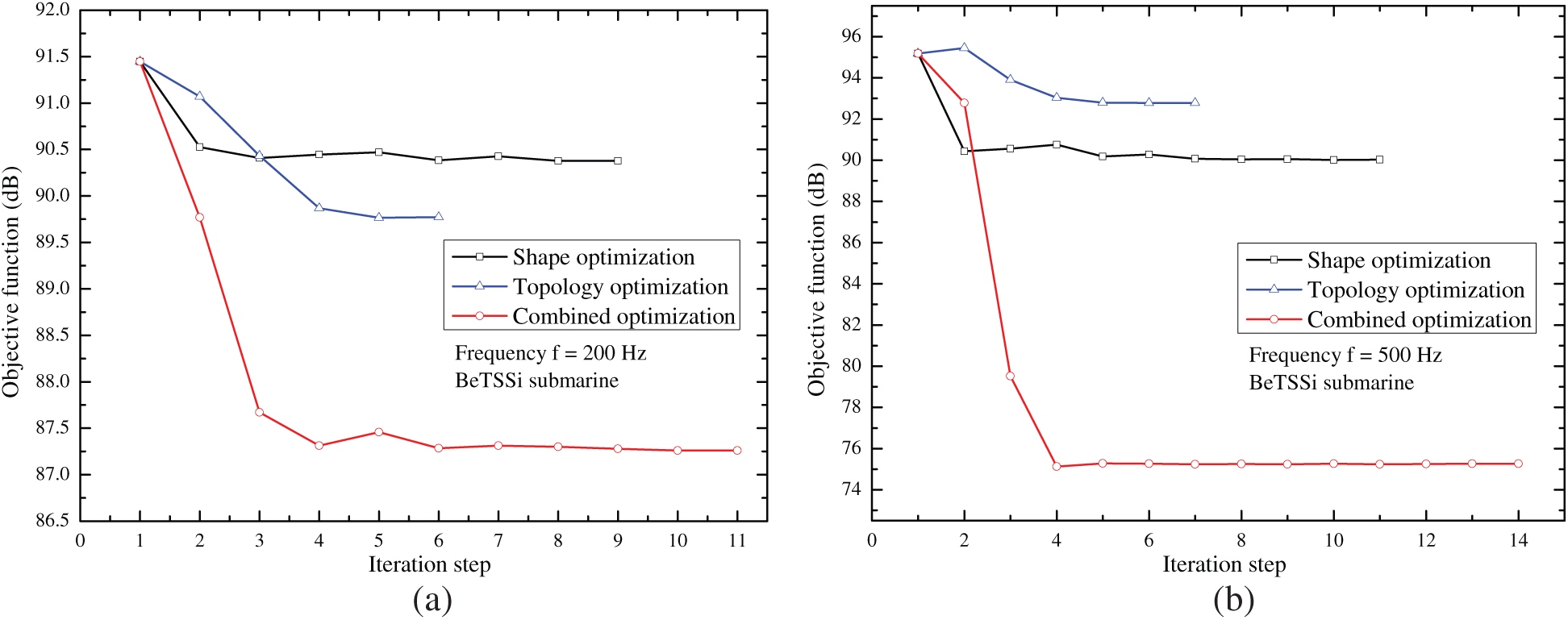
Figure 23: Iteration histories of objective function of BeTSSi submarine using three optimization methods (a) Frequency
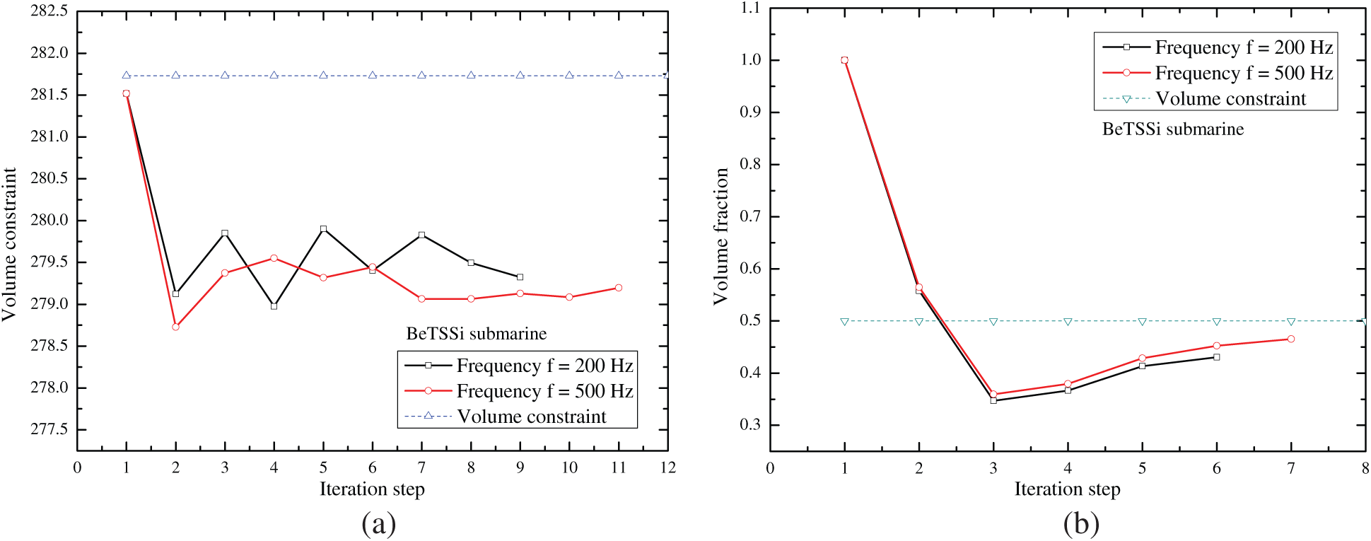
Figure 24: Iteration histories of BeTSSi submarine’s volume constraint for shape optimization and topology optimization (a) Shape optimization (b) Topology optimization
Figs. 25–28 show the optimization results for the submarine through the three optimization methods at frequency
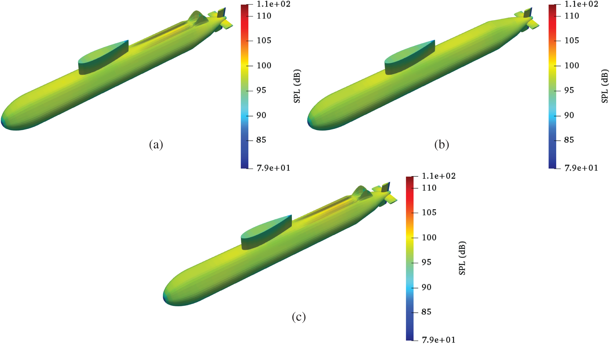
Figure 25: Surface SPL of optimized structure via three optimization methods at frequency
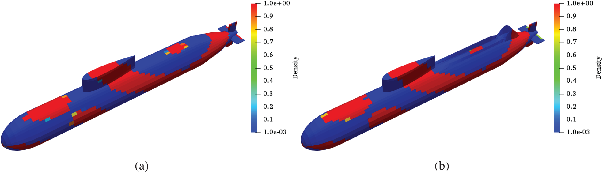
Figure 26: Distribution of SAM after optimization at frequency
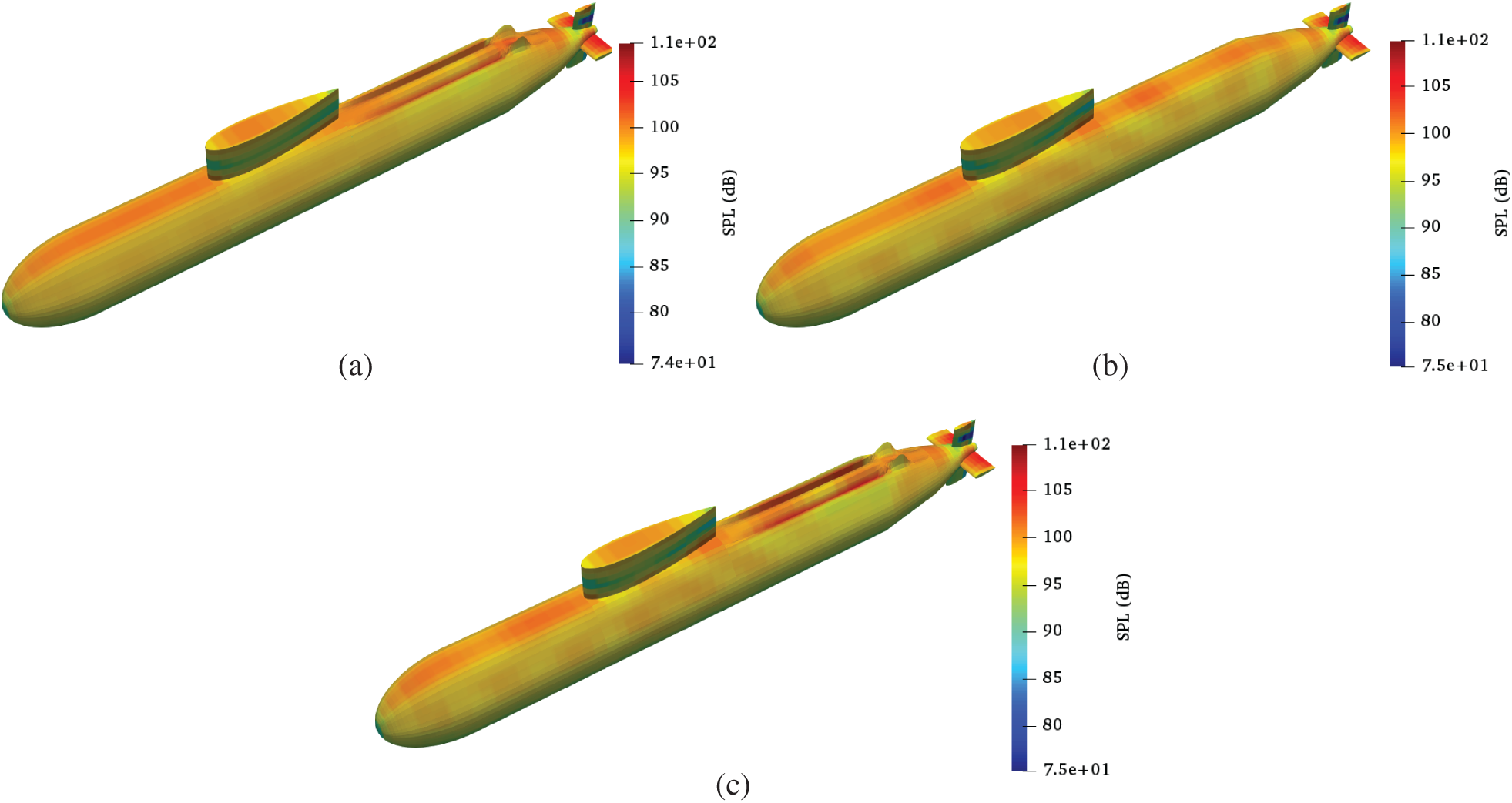
Figure 27: Surface SPL of optimized structure via three optimization methods at frequency
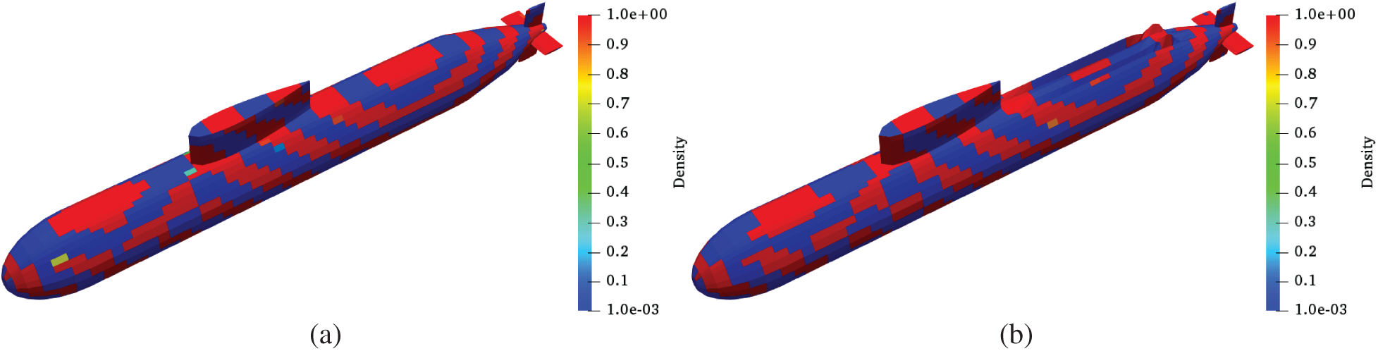
Figure 28: Distribution of SAM after optimization at frequency
In this study, we developed a combined shape and topology optimization algorithm for 3D structures based on IGA BEM. Different from the past shape optimization method on rigid structures, the impedance boundary condition is applied to the optimization process, where the structure surfaces are covered with SAM with artificial densities. The NURBS model constructs a bridge between geometry and physics, when surface shapes and the distribution of material change in each optimization iteration step. The control points are selected as the design parameters for shape optimization on account of their convenience and flexibility in shape control. With the application of SIMP method, the artificial densities of SAM located in integral elements are set as the design variables for topology optimization. The AVM is applied to the sensitivity analysis with respect to shape design parameters and topology design variables. Considering the computational efficiency and features of the two types of optimization, an iteration scheme for combined optimization, including a convergent topology optimization and a one-step shape optimization, is investigated in this study. Several numerical examples, including a complex submarine scattering model, are performed to demonstrate the potential of the proposed combined optimization in achieving improved noise reduction, compared with the single type of shape optimization or topology optimization. All the optimization processes obtain frequency-dependent results, where the optimized shape and distribution of material at higher frequency tend to show a better noise reduction.
In the future, we aim to apply the fast multipole method to the acoustic analysis and sensitivity analysis to expand the developed method to larger-scale engineering problems. The level set method is also considered replacing the SIMP method in topology optimization to eliminate the medium densities in the distribution of SAM.
Funding Statement: This study was financially supported by the National Natural Science Foundation of China (NSFC) under Grant No. 11772322, and the Strategic Priority Research Program of the Chinese Academy of Sciences under Grant No. XDB22040502.
Conflicts of Interest: The authors declare that they have no conflicts of interest to report regarding the present study.
1. Hughes, T. J., Cottrell, J. A., Bazilevs, Y. (2005). Isogeometric analysis: CAD, finite elements, NURBS, exact geometry and mesh refinement. Computer Methods in Applied Mechanics and Engineering, 194(39–41), 4135–4195. DOI 10.1016/j.cma.2004.10.008. [Google Scholar] [CrossRef]
2. Moheit, L., Marburg, S. (2018). Normal modes and modal reduction in exterior acoustics. Journal of Theoretical and Computational Acoustics, 26(3), 1850029. DOI 10.1142/S2591728518500299. [Google Scholar] [CrossRef]
3. Brebbia, C. A., Dominguez, J., Tassoulas, J. L. (1991). Boundary elements: An introductory course. Journal of Applied Mechanics, 58(3), 860. DOI 10.1115/1.2897280. [Google Scholar] [CrossRef]
4. Zheng, C., Matsumoto, T., Takahashi, T., Chen, H. (2012). A wideband fast multipole boundary element method for three dimensional acoustic shape sensitivity analysis based on direct differentiation method. Engineering Analysis with Boundary Elements, 36(3), 361–371. DOI 10.1016/j.enganabound.2011.09.001. [Google Scholar] [CrossRef]
5. Peters, H., Marburg, S., Kessissoglou, N. (2012). Structural-acoustic coupling on non-conforming meshes with quadratic shape functions. International Journal for Numerical Methods in Engineering, 91(1), 27–38. DOI 10.1002/nme.4251. [Google Scholar] [CrossRef]
6. Zhao, W., Zheng, C., Liu, C., Chen, H. (2018). Minimization of sound radiation in fully coupled structural-acoustic systems using FEM-BEM based topology optimization. Structural and Multidisciplinary Optimization, 58(1), 115–128. DOI 10.1007/s00158-017-1881-3. [Google Scholar] [CrossRef]
7. Bebendorf, M. (2000). Approximation of boundary element matrices. Numerische Mathematik, 86(4), 565–589. DOI 10.1007/PL00005410. [Google Scholar] [CrossRef]
8. Liu, Y., Nishimura, N. (2006). The fast multipole boundary element method for potential problems: A tutorial. Engineering Analysis with Boundary Elements, 30(5), 371–381. DOI https://dx.doi.org/10.1016/j.enganabound.2005.11.006. [Google Scholar]
9. Takahashi, T., Matsumoto, T. (2012). An application of fast multipole method to isogeometric boundary element method for Laplace equation in two dimensions. Engineering Analysis with Boundary Elements, 36(12), 1766–1775. DOI 10.1016/j.enganabound.2012.06.004. [Google Scholar] [CrossRef]
10. Wilkes, D. R., Peters, H., Croaker, P., Marburg, S., Duncan, A. J. et al. (2017). Non-negative intensity for coupled fluid-structure interaction problems using the fast multipole method. Journal of the Acoustical Society of America, 141(6), 4278–4288. DOI 10.1121/1.4983686. [Google Scholar] [CrossRef]
11. Dölz, J., Harbrecht, H., Kurz, S., Schöps, S., Wolf, F. (2018). A fast isogeometric BEM for the three dimensional Laplace-and Helmholtz problems. Computer Methods in Applied Mechanics and Engineering, 330(Suppl. C), 83–101. DOI 10.1016/j.cma.2017.10.020. [Google Scholar] [CrossRef]
12. Chen, L., Zheng, C., Chen, H. (2013). A wideband FMBEM for 2D acoustic design sensitivity analysis based on direct differentiation method. Computational Mechanics, 52(3), 631–648. DOI 10.1007/s00466-013-0836-9. [Google Scholar] [CrossRef]
13. Wang, J., Zheng, C., Chen, L., Chen, H. (2020). Acoustic shape optimization based on isogeometric wideband fast multipole boundary element method with adjoint variable method. Journal of Theoretical and Computational Acoustics, 28(2), 2050015. DOI 10.1142/S2591728520500152. [Google Scholar] [CrossRef]
14. Gu, J., Zhang, J., Li, G. (2012). Isogeometric analysis in BIE for 3-D potential problem. Engineering Analysis with Boundary Elements, 36(5), 858–865. DOI 10.1016/j.enganabound.2011.09.018. [Google Scholar] [CrossRef]
15. Taus, M., Rodin, G. J., Hughes, T. J. (2016). Isogeometric analysis of boundary integral equations: High-order collocation methods for the singular and hyper-singular equations. Mathematical Models and Methods in Applied Sciences, 26(8), 1447–1480. DOI 10.1142/S0218202516500354. [Google Scholar] [CrossRef]
16. Gong, Y., Dong, C., Qin, X. (2017). An isogeometric boundary element method for three dimensional potential problems. Journal of Computational and Applied Mathematics, 313, 454–468. DOI 10.1016/j.cam.2016.10.003. [Google Scholar] [CrossRef]
17. Chen, L., Li, K., Peng, X., Lian, H., Lin, X., et al. (2021). Isogeometric boundary element analysis for 2D transient heat conduction problem with radial integration method. Computer Modeling in Engineering & Sciences, 126(1), 125–146. DOI 10.32604/cmes.2021.012821. [Google Scholar] [CrossRef]
18. Simpson, R. N., Bordas, S. P., Trevelyan, J., Rabczuk, T. (2012). A two-dimensional isogeometric boundary element method for elastostatic analysis. Computer Methods in Applied Mechanics and Engineering, 209(11), 87–100. DOI 10.1016/j.cma.2011.08.008. [Google Scholar] [CrossRef]
19. Simpson, R. N., Bordas, S. P., Lian, H., Trevelyan, J. (2013). An isogeometric boundary element method for elastostatic analysis: 2D implementation aspects. Computers & Structures, 118(3), 2–12. DOI 10.1016/j.compstruc.2012.12.021. [Google Scholar] [CrossRef]
20. Li, S., Trevelyan, J., Zhang, W., Wang, D. (2018). Accelerating isogeometric boundary element analysis for 3-dimensional elastostatics problems through black-box fast multipole method with proper generalized decomposition. International Journal for Numerical Methods in Engineering, 114(9), 975–998. DOI 10.1002/nme.5773. [Google Scholar] [CrossRef]
21. Simpson, R. N., Scott, M. A., Taus, M., Thomas, D. C., Lian, H. (2014). Acoustic isogeometric boundary element analysis. Computer Methods in Applied Mechanics and Engineering, 269(139), 265–290. DOI 10.1016/j.cma.2013.10.026. [Google Scholar] [CrossRef]
22. Venås, J. V., Kvamsdal, T. (2020). Isogeometric boundary element method for acoustic scattering by a submarine. Computer Methods in Applied Mechanics and Engineering, 359(39–41), 112670. DOI 10.1016/j.cma.2019.112670. [Google Scholar] [CrossRef]
23. Wu, Y., Dong, C., Yang, H. (2020). Isogeometric indirect boundary element method for solving the 3D acoustic problems. Journal of Computational and Applied Mathematics, 363(3), 273–299. DOI 10.1016/j.cam.2019.06.013. [Google Scholar] [CrossRef]
24. Chen, L., Zhang, Y., Lian, H., Atroshchenko, E., Ding, C. et al. (2020). Seamless integration of computer-aided geometric modeling and acoustic simulation: Isogeometric boundary element methods based on Catmull-Clark subdivision surfaces. Advances in Engineering Software, 149(2), 102879. DOI 10.1016/j.advengsoft.2020.102879. [Google Scholar] [CrossRef]
25. Yang, H., Dong, C., Wu, Y. (2020). Non-conforming interface coupling and symmetric iterative solution in isogeometric FE-BE analysis. Computer Methods in Applied Mechanics and Engineering, 373(39), 113561. DOI 10.1016/j.cma.2020.113561. [Google Scholar] [CrossRef]
26. Ishizuka, T., Fujiwara, K. (2004). Performance of noise barriers with various edge shapes and acoustical conditions. Applied Acoustics, 65(2), 125–141. DOI 10.1016/j.apacoust.2003.08.006. [Google Scholar] [CrossRef]
27. Fard, S. M., Peters, H., Kessissoglou, N., Marburg, S. (2015). Three-dimensional analysis of a noise barrier using a quasi-periodic boundary element method. Journal of the Acoustical Society of America, 137(6), 3107–3114. DOI 10.1121/1.4921266. [Google Scholar] [CrossRef]
28. Baulac, M., Defrance, J., Jean, P. (2007). Optimization of multiple edge barriers with genetic algorithms coupled with a Nelder-Mead local search. Journal of Sound and Vibration, 300(1–2), 71–87. DOI 10.1016/j.jsv.2006.07.030. [Google Scholar] [CrossRef]
29. Chen, L., Zhao, W., Yuan, X., Zhou, B. (2018). Study on the optimization of the distribution of absorbing material on a noise barrier. Acoustics Australia, 46(1), 119–130. DOI 10.1007/s40857-017-0123-6. [Google Scholar] [CrossRef]
30. Zhao, W., Zheng, C., Chen, H. (2019). Acoustic topology optimization of porous material distribution based on an adjoint variable FMBEM sensitivity analysis. Engineering Analysis with Boundary Elements, 99(1–2), 60–75. DOI 10.1016/j.enganabound.2018.11.003. [Google Scholar] [CrossRef]
31. Zhao, W., Chen, L., Chen, H., Marburg, S. (2019). Topology optimization of exterior acoustic-structure interaction systems using the coupled FEM-BEM method. International Journal for Numerical Methods in Engineering, 119(5), 404–431. DOI 10.1002/nme.6055. [Google Scholar] [CrossRef]
32. Liu, C., Chen, L., Zhao, W., Chen, H. (2017). Shape optimization of sound barrier using an isogeometric fast multipole boundary element method in two dimensions. Engineering Analysis with Boundary Elements, 85, 142–157. DOI 10.1016/j.enganabound.2017.09.009. [Google Scholar] [CrossRef]
33. Chen, L., Liu, C., Zhao, W., Liu, L. (2018). An isogeometric approach of two dimensional acoustic design sensitivity analysis and topology optimization analysis for absorbing material distribution. Computer Methods in Applied Mechanics and Engineering, 336(39), 507–532. DOI 10.1016/j.cma.2018.03.025. [Google Scholar] [CrossRef]
34. Nørtoft, P., Gravesen, J. (2013). Isogeometric shape optimization in fluid mechanics. Structural and Multidisciplinary Optimization, 48(5), 909–925. DOI 10.1007/s00158-013-0931-8. [Google Scholar] [CrossRef]
35. Lee, S. W., Lee, J., Cho, S. (2015). Isogeometric shape optimization of ferromagnetic materials in magnetic actuators. IEEE Transactions on Magnetics, 52(2), 1–8. [Google Scholar]
36. Kostas, K., Fyrillas, M., Politis, C., Ginnis, A., Kaklis, P. (2018). Shape optimization of conductive-media interfaces using an IGA-BEM solver. Computer Methods in Applied Mechanics and Engineering, 340, 600–614. DOI 10.1016/j.cma.2018.06.019. [Google Scholar] [CrossRef]
37. Kostas, K., Ginnis, A., Politis, C., Kaklis, P. (2015). Ship-hull shape optimization with a T-spline based BEM-isogeometric solver. Computer Methods in Applied Mechanics and Engineering, 284(5–8), 611–622. DOI 10.1016/j.cma.2014.10.030. [Google Scholar] [CrossRef]
38. Lian, H., Kerfriden, P., Bordas, S. P. (2016). Implementation of regularized isogeometric boundary element methods for gradient-based shape optimization in two-dimensional linear elasticity. International Journal for Numerical Methods in Engineering, 106(12), 972–1017. DOI 10.1002/nme.5149. [Google Scholar] [CrossRef]
39. Lian, H., Kerfriden, P., Bordas, S. (2017). Shape optimization directly from CAD: An isogeometric boundary element approach using T-splines. Computer Methods in Applied Mechanics and Engineering, 317(4), 1–41. DOI 10.1016/j.cma.2016.11.012. [Google Scholar] [CrossRef]
40. Sun, D., Dong, C. (2020). Shape optimization of heterogeneous materials based on isogeometric boundary element method. Computer Methods in Applied Mechanics and Engineering, 370, 113279. DOI 10.1016/j.cma.2020.113279. [Google Scholar] [CrossRef]
41. Chen, L., Lian, H., Liu, Z., Chen, H., Atroshchenko, E. et al. (2019). Structural shape optimization of three dimensional acoustic problems with isogeometric boundary element methods. Computer Methods in Applied Mechanics and Engineering, 355(2), 926–951. DOI 10.1016/j.cma.2019.06.012. [Google Scholar] [CrossRef]
42. Chen, L., Lu, C., Lian, H., Liu, Z., Zhao, W. et al. (2020). Acoustic topology optimization of sound absorbing materials directly from subdivision surfaces with isogeometric boundary element methods. Computer Methods in Applied Mechanics and Engineering, 362(3–5), 112806. DOI 10.1016/j.cma.2019.112806. [Google Scholar] [CrossRef]
43. Zhuang, C., Xiong, Z., Ding, H. (2007). A level set method for topology optimization of heat conduction problem under multiple load cases. Computer Methods in Applied Mechanics and Engineering, 196(4–6), 1074–1084. DOI 10.1016/j.cma.2006.08.005. [Google Scholar] [CrossRef]
44. Matsumoto, T., Yamada, T., Takahashi, T., Zheng, C., Harada, S. (2011). Acoustic design shape and topology sensitivity formulations based on adjoint method and BEM. Computer Modeling in Engineering & Sciences, 78(2), 77–94. [Google Scholar]
45. Dunning, P. D., Alicia Kim, H. (2013). A new hole insertion method for level set based structural topology optimization. International Journal for Numerical Methods in Engineering, 93(1), 118–134. DOI 10.1002/nme.4384. [Google Scholar] [CrossRef]
46. Bendsøe, M. P., Sigmund, O. (1999). Material interpolation schemes in topology optimization. Archive of Applied Mechanics, 69(9–10), 635–654. DOI 10.1007/s004190050248. [Google Scholar] [CrossRef]
47. Christiansen, A. N., Nobel-Jørgensen, M., Aage, N., Sigmund, O., Bærentzen, J. A. (2014). Topology optimization using an explicit interface representation. Structural and Multidisciplinary Optimization, 49(3), 387–399. DOI 10.1007/s00158-013-0983-9. [Google Scholar] [CrossRef]
48. Christiansen, A. N., Bærentzen, J. A., Nobel-Jørgensen, M., Aage, N., Sigmund, O. (2015). Combined shape and topology optimization of 3D structures. Computers & Graphics, 46(2), 25–35. DOI 10.1016/j.cag.2014.09.021. [Google Scholar] [CrossRef]
49. Lian, H., Christiansen, A. N., Tortorelli, D. A., Sigmund, O., Aage, N. (2017). Combined shape and topology optimization for minimization of maximal von Mises stress. Structural and Multidisciplinary Optimization, 55(5), 1541–1557. DOI 10.1007/s00158-017-1656-x. [Google Scholar] [CrossRef]
50. Lin, W., Newman, J. C., Anderson, W. K., Zhang, X. (2017). Topology and shape optimization of broadband acoustic metamaterials and phononic crystals. Acoustical Science and Technology, 38(5), 254–260. DOI 10.1250/ast.38.254. [Google Scholar] [CrossRef]
51. Jiang, F., Zhao, W., Chen, L., Zheng, C., Chen, H. (2021). Combined shape and topology optimization for sound barrier by using the isogeometric boundary element method. Engineering Analysis with Boundary Elements, 124(2), 124–136. DOI 10.1016/j.enganabound.2020.12.009. [Google Scholar] [CrossRef]
52. Svanberg, K. (1987). The method of moving asymptotes-a new method for structural optimization. International Journal for Numerical Methods in Engineering, 24(2), 359–373. DOI 10.1002/nme.1620240207. [Google Scholar] [CrossRef]
53. Zhao, W., Chen, L., Zheng, C., Liu, C., Chen, H. (2017). Design of absorbing material distribution for sound barrier using topology optimization. Structural and Multidisciplinary Optimization, 56(2), 315–329. DOI 10.1007/s00158-017-1666-8. [Google Scholar] [CrossRef]
54. Zheng, C., Chen, H., Matsumoto, T., Takahashi, T. (2012). 3D acoustic shape sensitivity analysis using fast multipole boundary element method. International Journal of Computational Methods, 9(1), 1240004. DOI 10.1142/S021987621240004X. [Google Scholar] [CrossRef]
55. Chen, L., Marburg, S., Chen, H., Zhang, H., Gao, H. (2017). An adjoint operator approach for sensitivity analysis of radiated sound power in fully coupled structural-acoustic systems. Journal of Computational Acoustics, 25(1), 1750003. DOI 10.1142/S0218396X17500035. [Google Scholar] [CrossRef]
56. Zheng, C. J., Chen, H. B., Gao, H. F., Du, L. (2015). Is the Burton-Miller formulation really free of fictitious eigenfrequencies? Engineering Analysis with Boundary Elements, 59, 43–51. DOI 10.1016/j.enganabound.2015.04.014. [Google Scholar] [CrossRef]
57. Zheng, C. J., Bi, C. X., Zhang, C., Zhang, Y. B., Chen, H. B. (2019). Fictitious eigenfrequencies in the BEM for interior acoustic problems. Engineering Analysis with Boundary Elements, 104, 170–182. DOI 10.1016/j.enganabound.2019.03.042. [Google Scholar] [CrossRef]
58. Burton, A., Miller, G. (1971). The application of integral equation methods to the numerical solution of some exterior boundary-value problems. Proceedings of the Royal Society of London A, 323(1553), 201–210. [Google Scholar]
59. Marburg, S. (2016). The Burton and Miller method: Unlocking another mystery of its coupling parameter. Journal of Computational Acoustics, 24(1), 1550016. DOI 10.1142/S0218396X15500162. [Google Scholar] [CrossRef]
60. Guiggiani, M., Krishnasamy, G., Rudolphi, T. J., Rizzo, F. (1992). A general algorithm for the numerical solution of hypersingular boundary integral equations. Journal of Applied Mechanics, 59(3), 604–614. DOI 10.1115/1.2893766. [Google Scholar] [CrossRef]
61. Marburg, S. (2002). Developments in structural-acoustic optimization for passive noise control. Archives of Computational Methods in Engineering, 9(4), 291–370. DOI 10.1007/BF03041465. [Google Scholar] [CrossRef]
62. Merz, S., Kessissoglou, N., Kinns, R., Marburg, S. (2010). Minimisation of the sound power radiated by a submarine through optimisation of its resonance changer. Journal of Sound and Vibration, 329(8), 980–993. DOI 10.1016/j.jsv.2009.10.019. [Google Scholar] [CrossRef]
63. Zhang, Y., Wu, H., Jiang, W., Kessissoglou, N. (2017). Acoustic topology optimization of sound power using mapped acoustic radiation modes. Wave Motion, 70, 90–100. DOI 10.1016/j.wavemoti.2016.09.011. [Google Scholar] [CrossRef]
64. Wang, Y., Benson, D. (2015). Multi-patch nonsingular isogeometric boundary element analysis in 3D. Computer Methods in Applied Mechanics and Engineering, 293(41), 71–91. DOI 10.1016/j.cma.2015.03.016. [Google Scholar] [CrossRef]
65. Sun, Y., Trevelyan, J., Hattori, G., Lu, C. (2019). Discontinuous isogeometric boundary element (IGABEM) formulations in 3D automotive acoustics. Engineering Analysis with Boundary Elements, 105(5), 303–311. DOI 10.1016/j.enganabound.2019.04.011. [Google Scholar] [CrossRef]
Appendix A
The reconstructed BeTSSi submarine model consists of 7 NURBS patches, which are shown in Fig. 29.
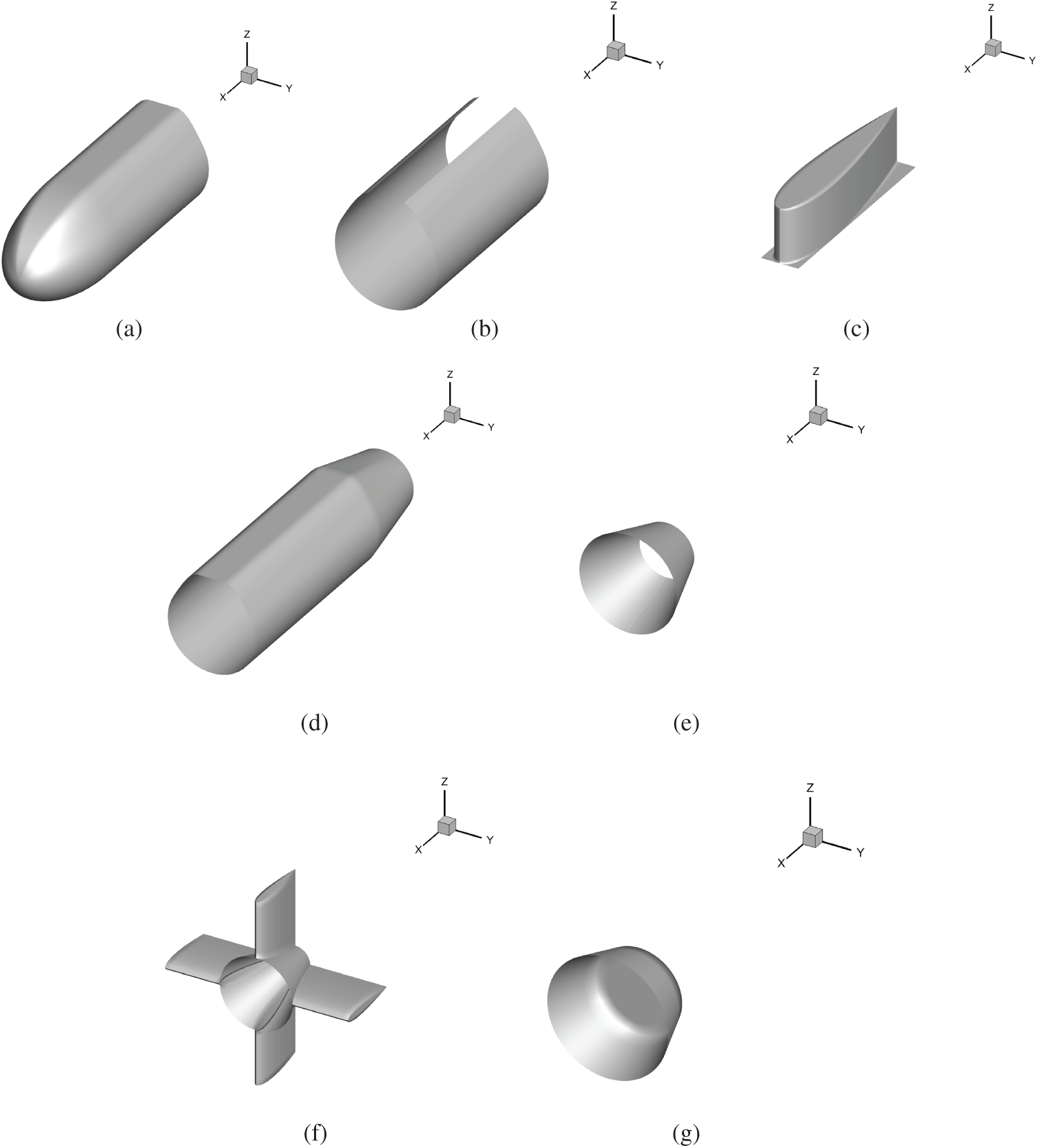
Figure 29: 7 NURBS patches of submarine model. (a) Patch 1. (b) Patch 2. (c) Patch 3. (d) Patch 4. (e) Patch 5. (f) Patch 6. (g) Patch 7
 | This work is licensed under a Creative Commons Attribution 4.0 International License, which permits unrestricted use, distribution, and reproduction in any medium, provided the original work is properly cited. |