Engineering & Sciences
| Computer Modeling in Engineering & Sciences |
DOI: 10.32604/cmes.2021.015153
ARTICLE
Modeling Additional Twists of Yarn Spun by Lateral Compact Spinning with Pneumatic Groove
1Key Laboratory of Textile Science & Technology, Ministry of Education, College of Textiles, Donghua University, Shanghai, 201620, China
2Merchandising and Digital Retailing, University of North Texas, Texas, 76203, USA
*Corresponding Authors: Longdi Cheng. Email: ldch@dhu.edu.cn; Bugao Xu. Email: bugao.xu@unt.edu
Received: 25 November 2020; Accepted: 26 February 2021
Abstract: Compact spinning with pneumatic grooves is a spinning process to gather fibers by blended actions of airflow and mechanical forces. Modified from the ring spinning system, the lateral compact spinning with pneumatic grooves can improve yarn appearance and properties due to generated additional twists. In this study, we investigated additional twists of the lateral compact spinning with pneumatic grooves via a finite element (FE) method. An elastic thin rod was used to model a fiber to simulate its dynamic deformation in the three-dimensional space, and the space bar unit was used to simplify the fiber model for the dynamic analysis. The stiffness equation of the elastic rod element and the dynamic equation of the rigid body mass element were derived from the differential equation of the elastic thin rod. In the analysis of the nonlinear geometric displacement of the space elastic thin rod unit, the large deformation problem was solved with the stepwise loading successive approximation. The simulation results explained the mechanism of generating additional twists, and the experiment results proved the existence of additional twists. The study demonstrated that the FE model is effective for predicting additional twists of fiber bundles in the agglomeration zone, and for simulating the fiber motion in the compact spinning with pneumatic grooves.
Keywords: Compact spinning; additional twist; finite element; dynamic analysis
Yarn twist, or the number of twists per unit length of yarn, directly affects yarn’s structure and mechanical properties, and fabric styles [1,2]. In studies of compact spinning, Zhou et al. [3,4] discovered twists in the condensing zone of pneumatic compact spinning with lattice aprons, and named these twists as “additional twists.” The reason why additional twists can be generated when a fiber bundle goes through the condensing zone is the force of lateral groove [5].
In order to study additional twists, Feldman [6] used material points as a fiber model to establish equations of the fiber motion in the condensing field and to obtain the trajectory of the fiber in a two-dimensional and non-uniform flow field. Bangert et al. [7] regarded fibers as rigid cylinders when describing motion and orientation of fibers under flow field forces. This was a relatively simple fiber model in the early time, which had drawbacks of no expression on the fiber rigidity. Jeffery [8] first proposed an orbital theory to solve the motion of a single rigid ellipsoid suspended in Newtonian fluid of a simple shear flow. Jeffery’s orbital theory has been widely used in subsequent fiber dynamics studies, and was enriched and perfected by Anezurowski et al. [9], Chiba et al. [10,11] and other researchers. In Jeffery’s orbital theory, the fiber was regarded as a rigid particle to represent the position and orientation of the fiber. However, this rigid particle was unable to reflect the flexibility and deformation of the fiber. Skjetne et al. [12] proposed a fiber model that consisted of a series of ellipsoids or spheres connected by “bead-bowl joints.” Nyland et al. [13] proposed a fiber model consisting of a plurality of rigid segments, which were connected by “bead-bowl joints.” Cheng [14,15] established a chain-ball model to analyze fiber motion with the movement patterns and deformations of fibers in incompressible viscous fluids. But Cheng’s model was too complex, and the viscoelastic property was not the main physical property of the fiber, although the research provided great inspiration and guidance for future studies on fiber models. Yamamoto et al. [16,17] proposed a bead-spring-chain model by arranging spheres connected by springs in series. Zeng et al. [18,19] treated a fiber as multiple elastic and flexible chains, and illustrated the elastic elongation of the fiber with changes in the mass point spacing of the chain. They also studied bending behaviors of the fiber with changes in the deflection of the chain. Wang [20] used a rigid micro-element segment as a fiber model to simulate the fiber motion in compact spinning with a lattice apron. The aforementioned fiber models regarded a fiber as multi-rigid chains to reflect the bending deformation characteristics, but these multi-rigid chains could not illustrate the elastic features of the fiber [21].
There is still a large gap between the performances of these existing fiber models and the actual mechanical behavior of a fiber. In this paper, we would like to introduce a continuous elastic thin rod to study the structure and dynamics of the fiber flexible body. The simultaneous partial differential equations of general nonlinear mechanics of the elastic thin rods are used to express the small deformation behavior of the rods. Based on the spatial elastic thin rod unit, we establish the fiber finite element (FE) model to explore the additional twists of lateral compact spinning with pneumatic grooves. The FE model of continuous elastic fine rods is used to simulate the fiber motion in compact spinning for both efficient calculations and effective visualization in the three-dimensional space. The FE method is applied to solving the dynamic problem of the large deformation of an elastic thin rod. The stiffness equation of the elastic rod element and the dynamic equation of the rigid body are derived from the dynamic analysis of a combination of mass units and elastic rod units. The nonlinear geometric large deformation problem of the spatial elastic thin rod unit is studied by solved the method of step-by-step loading and successive approximation. The goal of the research is to present an effective and feasible theoretical model and method for examining the twist formation process and mechanism of flexible fibers under the mechanical force of lateral grooves.
2.1 Establishment of Fiber Finite Element Model
Fig. 1a shows a roller system that draws and gather fiber bundles to form a desired yarn. And Figs. 1b and 1c are the groove shapes of the intermediate compact spinning with pneumatic groove and the lateral compact spinning with pneumatic groove.
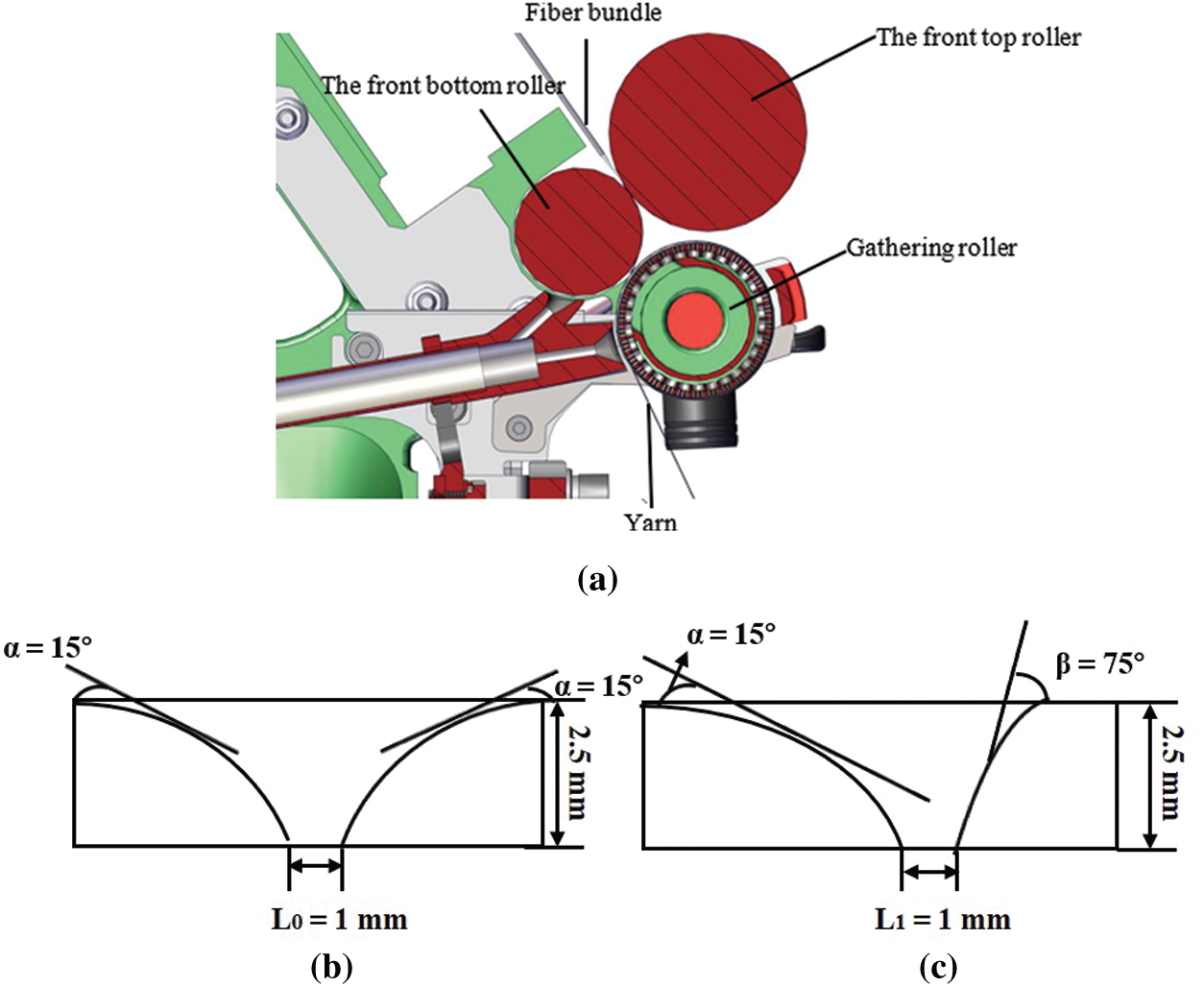
Figure 1: Diagram of compact spinning devices. (a) Gathering process of fiber bundle, (b) the intermediate compact spinning with pneumatic groove, (c) the lateral compact spinning with pneumatic groove
In order to solve the nonlinear large deformation problem and to realize the large draw ratio (fiber length/fiber diameter) of fibers, a finite element model is established with spatial elastic thin-rod units., as shown in Figs. 2 and 3. Fig. 2 presents the micro-segment rigid body of the FE model that shows the general motion of node i, while Fig. 3 displays elastic thin rods in the finite element model. In Fig. 2, O-xyz is an overall coordinate system, and O’-uvw is a connected moving coordinate system of a rigid body, or a local coordinate system. The origin of the coordinate is located at the centroid of the rigid body, and the direction of a coordinate axis is the direction of the principal axis of the mass center of the rigid body. The u axis is in the axial direction of the micro-segment, the v and w axes are located on the cross section of the micro-segment rigid body through the centroid.
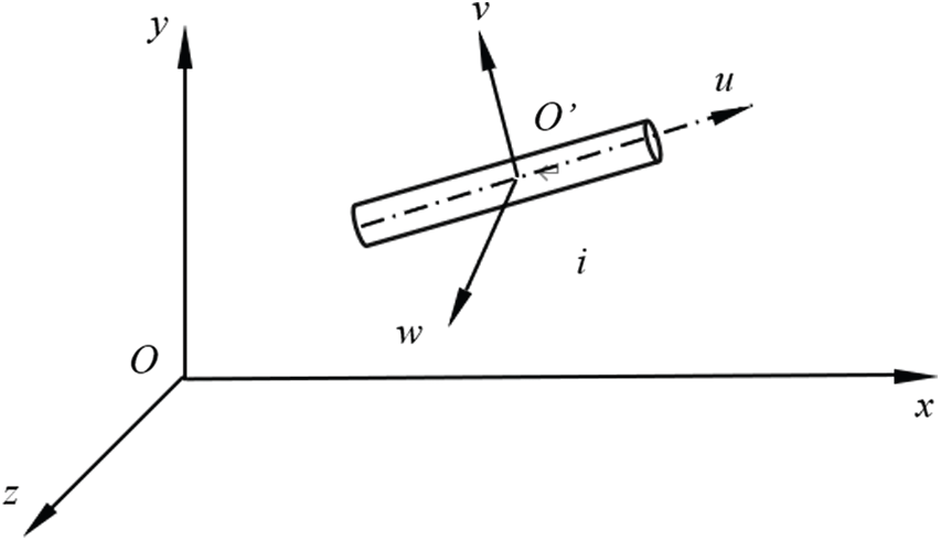
Figure 2: Rigid body unit for general motion in space
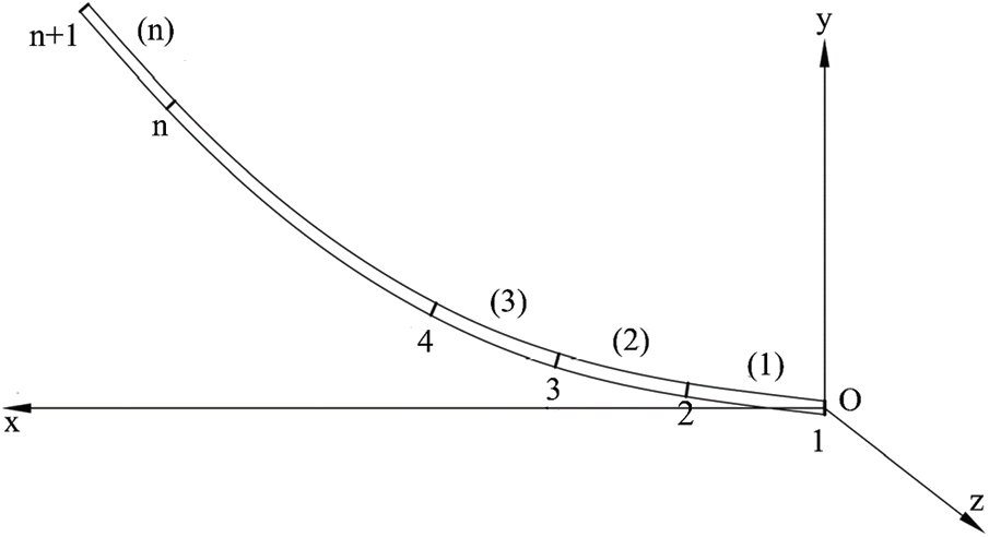
Figure 3: Elastic thin rods in the finite element model [22]
To analyze the dynamics of the elastic thin rod, the elastic thin rod is divided into n independent micro-segments and n + 1 nodes. Each node relative to the overall coordinate system has six degrees of freedom. Six coordinate parameters are needed to determine the relative position of a node. Three of the six parameters describe the moving line displacement of the node, and the other three describe the cross-sectional rotational angular displacement of the node. When the mass of the elastic thin rod is considered, the mass of each micro-segment is regarded as a rigid body moving with its local coordinate system (see Fig. 2). When the elasticity of the elastic thin rod is considered, the connection between two adjacent nodes is regarded as one elastic rod unit that is massless (see Fig. 3). The external force on the elastic thin rod is simplified so that it is only exerted on the two end nodes.
Any general motion of the rigid body in space can be decomposed into the translation with its centroid and the rotation relative to the centroid. According to the centroid motion theorem, the dynamic equation of the rigid body translation with centroid O’ is
where m is the mass of the rigid body,
According to the momentum quadrature theorem, the dynamic equation of the rigid body rotating around the centroid O’ can be derived as
where
In coordinate O-xyz, it can be simplified as:
where
Assume that the inertia of a micro rigid body relative to O’-uvw is
Then
where the direction cosine matrix of O’uvw relative to O-xyz is
The influence of the axial force on bending deformation must be considered in a large deformation of the elastic thin bar. The bending deformation of the elastic thin rod unit is shown in Fig. 4. Considering the influence of the rod axial force on the bending moment, the bending moment M of the rod element is
where v is the deflection of the rod, Fn is the rod axial force, and Fn = − Fui = Fuj.
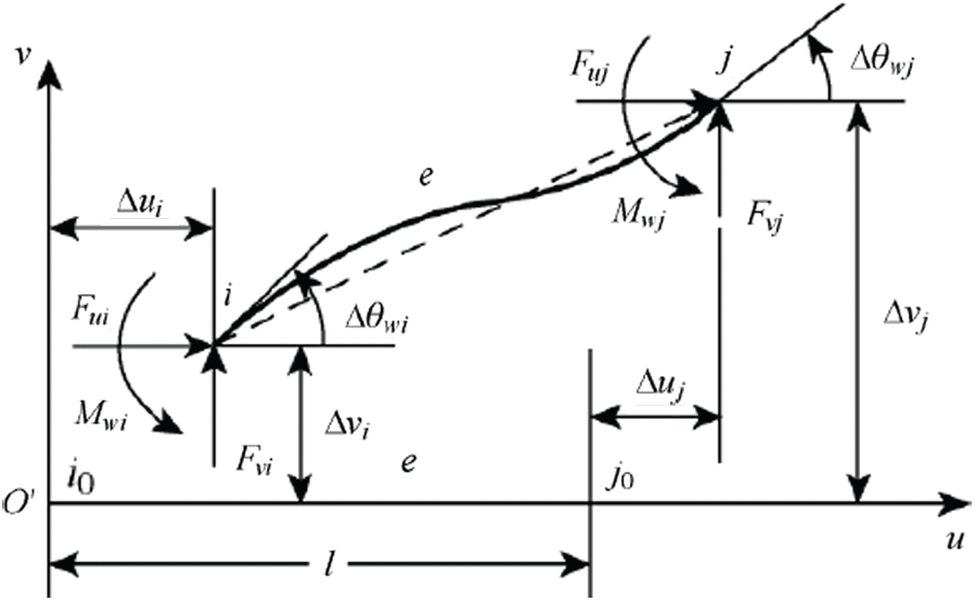
Figure 4: Bending deformation of the elastic thin rod unit
Given that the displacement of the rod element is small and in the limits of elastic deformation, plastic (unrecoverable) deformation can be ignored. The deflection of the rod v is
where l is the length of the rod unit.
If the displacement of the rod element is relatively small in the local coordinate system O’-uvw and the first derivative of the deflection is small, the differential equation of the rod bending deflection is
where E is the elastic modulus, and Iw is the section moment of inertia.
According to Eqs. (13) and (14) and the integral of u, the boundary condition of the rod element node and the balance equation of the rod element force, the matrix equation of the bending deformation of the elastic rod unit in the plane uO’v can be expressed as follows
Similarly, the bending deformation matrix equation of the elastic rod unit in the plane uO0w can be derived.
For the axial tension compression and torsion deformation of the rod unit, the following relationships can be derived
where G is the shear elastic modulus, A is the cross-sectional area, and Ip is polar moment of inertia of cross section. According to Eqs. (16) and (17), the stiffness matrix [k*] of the spatial bar element relative to the local coordinate system can be obtained.
Fig. 5 shows the elastic bar element in the local coordinate system, where i and j are the node positions of the elastic thin rod time t. The coordinate system of node i is taken as the local coordinate system of the unit, and the coordinate plane O’vw is called the cross section of node i, the
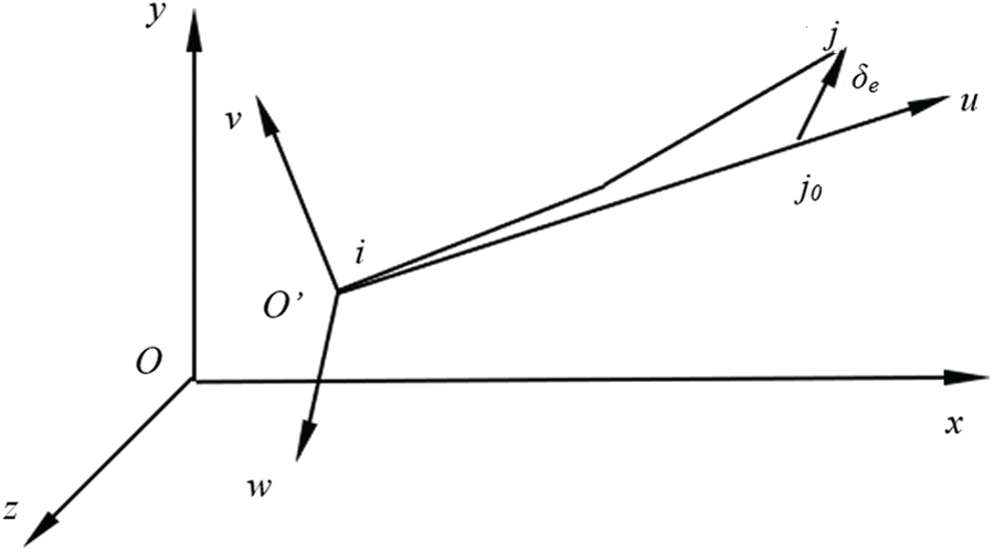
Figure 5: Elastic bar element and local coordinate system
The relationship between the deformation displacement of the elastic rod element and the force of the rod end relative to the overall coordinate system O-xyz can be expressed as
where the end force and deformation displacement of the element relative to O-xyz are
where
Taking the coordinate system O’-uvw of node i as the local coordinate system of the unit (see Fig. 4), then we have
Let
For the dynamic equation of all the nodes, Eq. (4) can be written in a matrix form as
where the vacancy element is zero, and
The dynamic equation of each elastic rod unit e can be written in a matrix form as
where
Substituting Eqs. (23) and (24) from Eq. (25), the new equation can be written as
where,
Eq. (26) is the differential equation describing motions of elastic thin rods for the FE dynamic analysis.
The differential equation of the dynamic FE model is solved by a specially developed MATLAB program to simulate the additional twists of yarn in the condensing zone. In the simulation, the ramie fiber was taken as an example where the fiber diameter along the fiber length was assumed to be uniform, the elastic modulus E of the fiber was 2224.6 cN/tex, and the shear elastic modulus G of the fiber was 106.2 cN/tex, the fiber diameter was 0.02 mm, the fiber density was 1.54 g/cm3, and the fiber length in the agglomeration area was 40 mm. The other parameters used in the analysis included the size of the fiber AB division unit of 0.5 mm, the number of fiber AB division units of 200, and the time integral step of 10−6. The gathering roller was made of rubber and supported by a copper sleeve, and thus the friction coefficient
When an edge fiber was connected with central fibers and the lateral pneumatic grooves, the contact was treated as a flexible connection constraint with sufficient stiffness in the simulation. Each node was subjected to the normal elastic connection occurring on the central cylinder, and the wall surface was constrained by the reaction force Fn. Its size was related to the normal spacing
where l was the unit length, and c was a sufficiently large stiffness factor (in this paper,
where f was the coefficient of sliding friction at the connect. The direction of friction was opposite to the direction of the node speed.
To implement the numerical calculation for the FE dynamic differential equations of the elastic thin rods, the implicit difference scheme Euler method was adopted. The calculation process was stable and the calculation results were reliable [23].
In order to solve the problem of large deformation, this paper adopts the load incremental step loading method. The load is divided into N loading steps from zero, which ensures that the load increment for each step is a small amount. For the first load step at which the load is zero, the position of the entire non-loaded state of the elastic rod unit is taken as the initial position. Establishing a local coordinate system at the initial position, the second step is taken. The displacement of each elastic rod unit under the load is solved by the element stiffness equation established under the small displacement condition, and the new position of the whole fiber after the first deformation will be obtained. For any N loading step calculation, the position of the elastic rod unit in step
Fig. 6 shows the path of a fiber bundle from the entering point A, the gathering roller, and to the exiting point B in the condensing zone. According to the specific value, the fiber motion in the agglomeration area was calculated by using the MATLAB software.
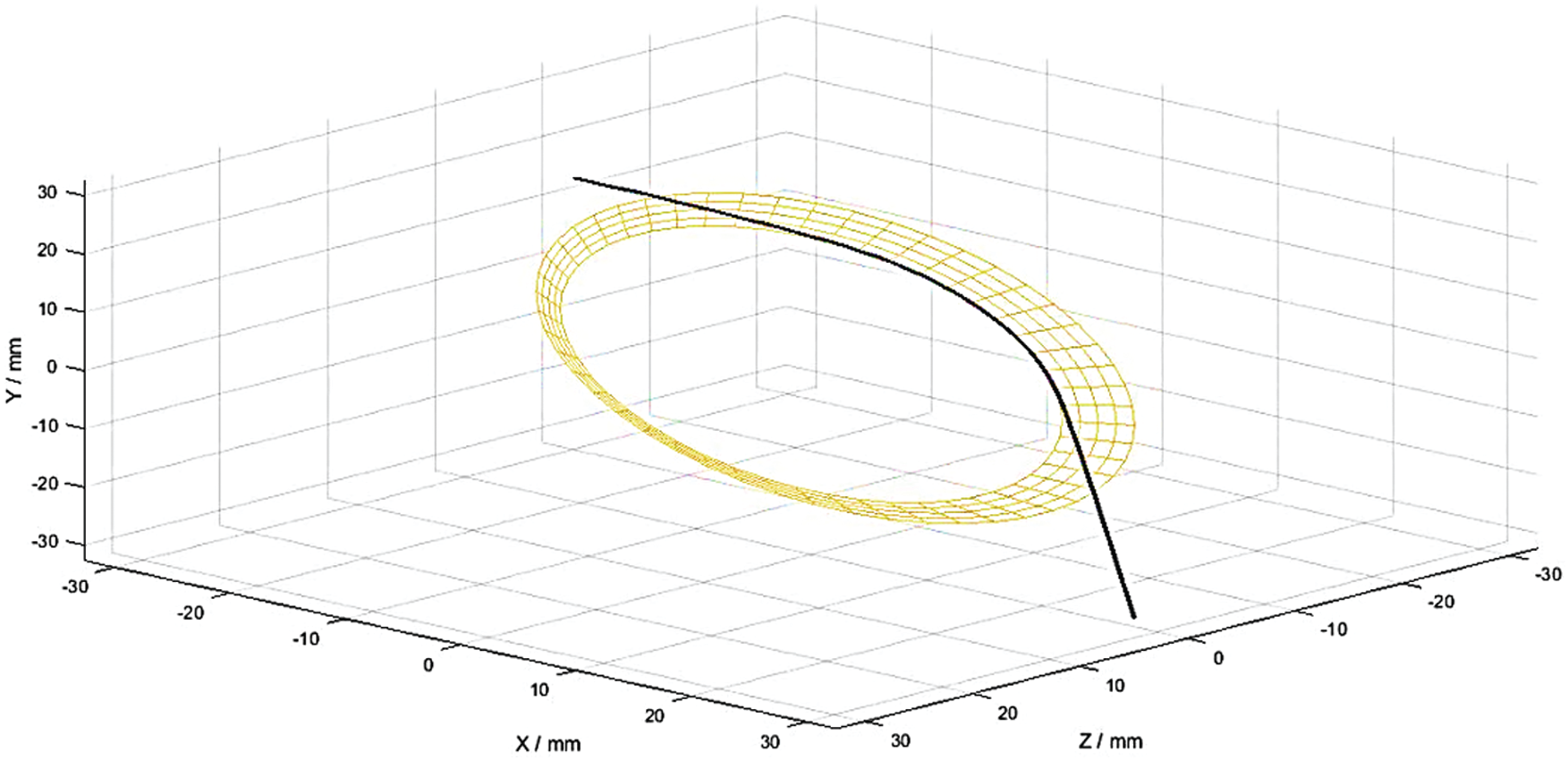
Figure 6: Fiber simulation model
Fig. 7 shows the movement of the fiber bundle. Fig. 7a is the simulation result of intermediate compact spinning with pneumatic grooves, while Fig. 7b is the simulation result of lateral compact spinning with pneumatic grooves. Figs. 7c and 7d are the fiber motion in the YZ plane of the two spinning systems. Unlike fibers in the intermediate compact spinning (Fig. 7c), fibers of the lateral compact spinning with pneumatic grooves had additional twists because fiber 5 crossed fiber 4 (Fig. 7d). Because of the lateral direction of fiber bundle in the agglomeration area, fibers, especially boundary fibers, would move closer to the center. The fiber bundle became more inseparable, which would improve yarn’s properties.
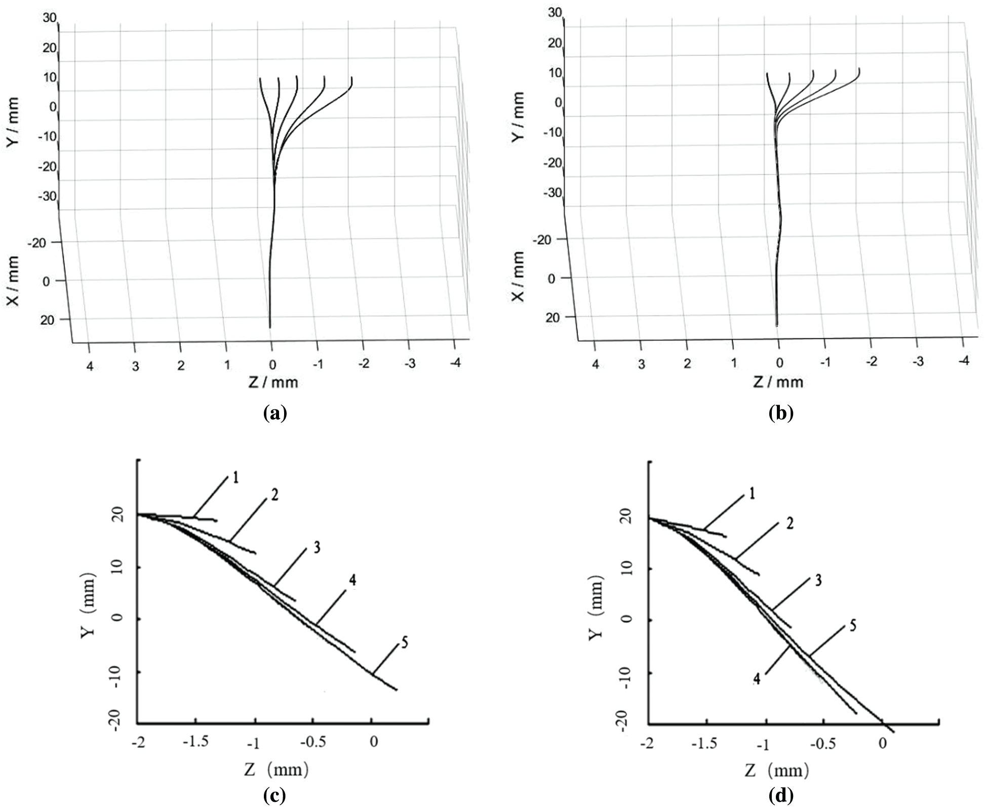
Figure 7: Fiber simulation results. (a): Fiber motion of intermediate compact spinning with pneumatic; (b): fiber motion of lateral compact spinning with pneumatic grooves; (c): YZ plane of fiber motion of intermediate compact spinning with pneumatic; (d): YZ plane of fiber motion of lateral compact spinning with pneumatic [22]
In order to determine the additional twist, yarns of the lateral compact spinning of pneumatic grooves were spun and compared with the intermediate compact spinning with pneumatic grooves yarns. The raw material was ramie roving. The roving linear density was 4.70 g/10 m, and the moisture regain of the roving was 12.0%. All the spinning was finished by the FZ501 spinning machine. The pressure of pneumatic grooves was −2600 (Pa), the twist was 680 (T/m), the spinning speed was 7000 (r/min), and the count of yarn was 36 Nm.
The tests were performed in the standard climate where the relative humidity was

In the paired
Fig. 8 shows yarn forms of the two different spinning methods. The quality of the yarn made from the lateral compact spinning with pneumatic grooves is better than that from the intermediate compact spinning. The yarn in Fig. 8a appears to be less hairy and tighter due to additional twists than the yarn in Fig. 8b. Therefore, the lateral compact spinning yarns possess better shape and mechanical performance.

Figure 8: Yarn of two spinning systems: (a): yarn of lateral entry compact spinning with pneumatic grooves; (b): yarn of intermediate compact spinning with pneumatic grooves
This paper provided a theoretical method for modeling the dynamic motion that simulates fibers driven by mechanical forces in the lateral compact spinning. In the study, we established a fiber FE model to simulate the large deformation process of the elastic thin rod element, and deduced the dynamic equilibrium equation of the spatial elastic thin rod unit in the model. We numerically obtained the movements of fibers under agglomeration and visually displayed additional twists generated in the lateral compact spinning with pneumatic grooves. The experiments demonstrated that the lateral compact spinning could produce smoother and tighter yarns that the intermediate compact spinning due to additional twists. Thus, the fiber FE model may be used to solve the large deformation problem of fiber motion in the three-dimensional space.
Funding Statement: This work is supported in part by China Scholarship Council and National Key R&D Program of China (Grant No. 2017YFB0309100).
Conflicts of Interest: The authors declare that they have no conflicts of interest to report regarding the present study.
1. Yu, C. W. (2009). Spinning. CN: China Textile Press. [Google Scholar]
2. Yu, C. W. (2010). Spinning. CN: China Textile Press. [Google Scholar]
3. Zhou, S. P., Wang, J., Yang, J. P. (2005). Mechanical analysis of sections of straight sections in the compact field. Donghua University (Nature Science), 31(2), 20–23. DOI 10.3969/j.issn.1671-0444.2005.02.006. [Google Scholar] [CrossRef]
4. Zhou, S. P., Wang, J., Yang, J. P. (2005). Mechanical analysis of sections of straight sections in the compact field. Donghua University (Nature Science), 31(3), 10–14. DOI 10.3969/j.issn.1671-0444. [Google Scholar] [CrossRef]
5. Yang, X., Wang, J., Yang, J. P. (2003). Development status and prospects of concentrated spinning. Donghua University (Nature Science), 329(2), 105–110. DOI 10.3969/j.issn.1671-0444.2003.02.024. [Google Scholar] [CrossRef]
6. Feldman, L. (1996). Theoretical trajectory studies of light bodies in non-uniform two-dimensional flows. Textile Research Journal, 36(9), 809–813. DOI 10.1177/004051756603600907. [Google Scholar] [CrossRef]
7. Bangert, L. H., Sagdeo, P. M. (1997). On fiber alignment using fluid-dynamic forces. Textile Research Journal, 47(12), 773–780. DOI 10.1177/004051757704701203. [Google Scholar] [CrossRef]
8. Jeffery, G. B. (1922). The motion of ellipsoid particles immersed in a viscous fluid. Proceedings of The Royal Society A-Mathematical Physical and Engineering Sciences, 102, 161–179. DOI 10.1098/rspa.1922.0078. [Google Scholar] [CrossRef]
9. Anezurowski, E., Mason, S. G. (1967). The kinetics of flowing dispersions: Equilibrium orientations for rods and dices (theoretical). Journal of Colloid and Interface Science, 23(4), 522–532. DOI 10.1016/0021-9797(67)90199-3. [Google Scholar] [CrossRef]
10. Chiba, K., Nakamura, K. (1998). Numerical solution of fiber suspension flow through a complex channel. Journal of Nanonewton Fluid, 78(2–3), 167–185. DOI 10.1016/S0377-0257(98)00067-6. [Google Scholar] [CrossRef]
11. Chiba, K., Komatsu, T. (2007). Numerical simulation for orientation of thin disk particles in a Newtonian flow through an L-shape channel. Journal of Textile Engineering, 53(1), 31–35. DOI 10.4188/jte.53.31. [Google Scholar] [CrossRef]
12. Skjetne P., Ross R. F., Klingenberg D. J. (1997). Simulation of single fiber dynamics. Journal of Chemical Physics, 107(6), 2108–2121. DOI 10.1063/1.474561. [Google Scholar] [CrossRef]
13. Nyland, G. H., Skjetne, P., Mikkelsen, A., Elgsaeter, A. (1996). Brownian dynamics simulation of needle chains. Journal of Chemical Physics, 105(3), 1198–1207. DOI 10.1063/1.471941. [Google Scholar] [CrossRef]
14. Cheng, D. W. (1987). Discrimination of the plane motion of curved fiber. Donghua University, 13(6), 73–77. DOI CNKI:SUN:DHDZ.0.1987-06-010. [Google Scholar]
15. Cheng, D. W. (1998). Suspension dynamics of viscoelastic fibers in a uniform deformation flow field. Donghua University, 14(6), 89–96. DOI CNKI:SUN:DHDZ.0.1988-06-014. [Google Scholar]
16. Yamamoto, S. M. (1993). A method for dynamic simulation of rigid and flexible fibers in a flow field. Journal of Chemical Physics, 98(1), 644–650. DOI 10.1063/1.464607. [Google Scholar] [CrossRef]
17. Yamamoto, S. M. (1994). The viscosity of dilute suspensions of rod like particles: A numerical simulation method. Journal of Chemical Physics, 100(4), 3317–3324. DOI 10.1063/1.466423. [Google Scholar] [CrossRef]
18. Zeng, Y. C., Yu, C. W. (2003). A bead-elastic rod model for dynamic simulation of fibers in high-speed air flow. International Journal of Nonlinear Science and Numerical Simulation, 4(2), 201–202. DOI 10.1515/IJNSNS.2003.4.2.201. [Google Scholar] [CrossRef]
19. Zeng, Y. C. (2003). Research and application of fiber movement in nozzle high-speed airflow, (Ph.D. Thesis). Donghua University, China. [Google Scholar]
20. Wang, Y. (2010). Study on aggregation mechanism and yarn performance of grid-type compact aggregate spinning, (Ph.D. Thesis). Donghua University, China. [Google Scholar]
21. Liu, Y. Z. (2006). Nonlinear mechanics of elastic thin rods. CN: Tsinghua University Press. [Google Scholar]
22. Lyu, J. D., Cheng, L. D., Xu, B. G., Hua, Z. H. (2021). Numerical simulation of fiber motion of lateral compact spinning with pneumatic groove. Autex Research Journal, (In press). [Google Scholar]
23. Jiang, J. F., Hu, L. J., Tang, J. (2004). Numerical analysis and matlab experiment. CN: Science Press. [Google Scholar]
24. Huo, S. H. (2001). GB/T 2543.2-2001. Textiles-determination of twist in yarn-part2: Untwist-retwist method. CN: China Standards Press. [Google Scholar]
 | This work is licensed under a Creative Commons Attribution 4.0 International License, which permits unrestricted use, distribution, and reproduction in any medium, provided the original work is properly cited. |