Computer Modeling in Engineering & Sciences

DOI: 10.32604/cmes.2021.014950

ARTICLE

Quadratic Finite Volume Element Schemes over Triangular Meshes for a Nonlinear Time-Fractional Rayleigh-Stokes Problem

Yanlong Zhang1, Yanhui Zhou2 and Jiming Wu3,*

1Graduate School of China Academy of Engineering Physics, Beijing, 100088, China
2School of Data and Computer Science, Sun Yat-Sen University, Guangzhou, 510275, China
3Institute of Applied Physics and Computational Mathematics, Beijing, 100088, China
*Corresponding Author: Jiming Wu. Email: wu_jiming@iapcm.ac.cn
Received: 11 November 2020; Accepted: 15 January 2021

1  Introduction

Recently, due to the widespread use of fractional partial differential equations (FPDEs), such as dispersion in a porous medium, statistical mechanics, mathematical biology and so on, numerical solution of FPDEs becomes one of the frontier fields in the research. Fractional partial differential equations can be roughly classified into three categories: Space FPDEs [1–10], time FPDEs [11–29] and space-time FPDEs [30–34]. Anomalous sub-diffusion equations, one type of time FPDEs, arise in some physical and biological processes. And the study of FPDEs with anomalous sub-diffusion terms, such as modified anomalous sub-diffusion equations [17,18], fractional Cable equations [11,16] or others, is also meaningful and popular. The problem considered in this article, which belongs to a nonlinear time-fractional Rayleigh-Stokes problem [19–22] applied in some non-Newtonian fluids, is a variant of the Stokes’ first problems and Rayleigh-Stokes problems [35–38], and it is important in physics and engineering.

At present, numerical simulation is an important and effective way to solve partial differential equations, and the relevant numerical methods can be finite difference methods [7,8,14–17], finite element methods (FEMs) [1,2,9,11–13,21,29,31–33,39], meshless methods [40,41], finite volume methods [3–6,42–54] and so on. Of course, the research for FPDEs by finite volume element methods (FVEMs) [10,23–28] has no exception for the local conservation and simple implementation. Sayevand et al. [23] presented a spatially semi-discrete piecewise linear FVEM for the time-fractional sub-diffusion problem and obtained some error estimates of the solution in both FEMs and FVEMs. A linear finite volume element scheme for the 2D time-fractional anomalous sub-diffusion equations was studied and analyzed by Karaa et al. [24], where the convergence rate was of order h2+Δt1+α in the L∞(L2) norm and the results were improved in [25] for both smooth and nonsmooth initial data. Badr et al. [26] proposed a linear FVEM for the time-fractional advection diffusion problem in one-dimension, and proved that the fully discrete scheme is unconditionally stable. Furthermore, Yazdani et al. [10] solved a space-fractional advection-dispersion problem in one-dimension by using linear FVEM and proved it is stable when the mesh grid size is small enough. Zhao et al. [27] constructed a mixed finite volume element scheme for the time-fractional reaction-diffusion equation, and showed the unconditional stability analysis for it. Moreover, Zhao et al. [28] proposed a linear FVEM for the nonlinear time-fractional mobile/immobile transport equations on triangular grids, and obtained the optimal priori error estimates in L∞(L2) and L2(H1) norms. To our knowledge, the study of high order finite volume element methods for 2D FPDEs is undiscovered.

There are some research about quadratic finite volume element methods for solving partial differential equations on triangular meshes. Tian et al. [42] presented quadratic element generalized differential methods to solve elliptic equations where two parameters of the quadratic element were β1=β2=1/3 (referring to the definition Eqs. (4), (5)). Liebau [43] solved one type of elliptic boundary value problems by a quadratic element scheme with parameters β1=1/4,β2=1/3, and proved 𝓞(h2) error estimate under some assumption conditions. Xu et al. [44] started to study the structure about two parameters of the quadratic element, and improved some existing coercivity results. Chen et al. [45] established a general framework for construction and analysis of the higher-order finite volume methods. Wang et al. [46] established a unified framework to perform the L2 error analysis for high order finite volume methods on triangular meshes, and proposed a new quadratic scheme with parameters β1=(3-3)/6,β2=(6+3-21+63)/9 to achieve the optimal L2 convergence order. An unconditionally stable quadratic finite volume scheme with parameters β1=β2=(3-3)/6 for elliptic equations was presented by Zou [47], and it had optimal convergence orders under H1 norms. For the quadratic finite volume element schemes with parameters β1=(3-3)/6,β2∈(0,2/3), Zhou et al. [48] obtained an analytic minimum angle condition and an optimal H1 error estimates under the improved coercivity result. Moreover, a unified framework for the coercivity analysis of a class of quadratic schemes with parameters β1∈(0,1/2),β2∈(0,2/3) was established for elliptic boundary value problems [49], which covered all the existing quadratic schemes of Lagrange type, and minimum angle conditions of the existing literatures are improved. All the above papers are mainly confined to the elliptic problems and we have seen some applications to other problems [50–53], but none relevant study for FPDEs.

In this article, the quadratic finite volume element method is proposed to solve one class of FPDEs, that is, a 2D nonlinear time-fractional Rayleigh-Stokes problem with the time-fractional derivative defined by Caputo fractional derivative. In spatial direction, this problem is solved by a class of quadratic finite volume element schemes with two parameters β1 and β2. Moreover, this problem is discretized at time tn-α/2 and the time-fractional derivative is discretized through L2-1σ formula in time direction. Numerical experiments indicate the efficiency of the schemes, specifically, the L2 error estimate of one scheme is 𝓞(h3+Δt2), and L2 error estimates of other schemes are 𝓞(h2+Δt2). We find that the new finite volume element schemes are comparable with an existing finite element scheme [29].

The outline of this paper is as follows. In Section 2, we describe in details the specific algorithm steps of the quadratic finite volume element schemes over triangular meshes, and finally obtain the fully discrete schemes. In Section 3, some numerical experiments are performed to investigate the performance of the quadratic finite volume element schemes. The numerical results are also compared with those of an existing quadratic finite element scheme. A brief conclusion ends this article in last section.

2  Quadratic Finite Volume Element Schemes

2.1 Preliminary

In this article, we construct a family of quadratic finite volume element schemes to solve the following 2D nonlinear time-fractional Rayleigh-Stokes problem:

∂u(x,t)∂t−∂αΔu(x,t)∂tα−Δu(x,t)=f(u)+g(x,t), (x,t)∈Ω×(0,T], (1)

u(x,t)=0, (x,t)∈∂Ω×(0,T], (2)

u(x,0)=u0(x), x∈Ω, (3)

where x=(x,y)∈Ω⊂ℝ2 and ∂αΔu(x,t)∂tα=1Γ(1-α)∫0t∂Δu(x,τ)∂τdτ(t-τ)α, denotes the Caputo fractional derivative of order α∈(0,1), which is an anomalous sub-diffusion term. f(u) is a nonlinear term subjected to the following conditions, |f(u)|≤C1|u| and |f′(u)|≤C2 where C1 and C2 are positive constants, and g(x,t) is the source term.

For the numerical solution of Eqs. (1)–(3), the space domain Ω is first triangulated to get the so-called primary mesh 𝓒h, see the solid line segments in Fig. 1. The trial function space Uh is then defined with respect to 𝓒h, given by Uh={uh∈C(Ω̄):uh∣K∈ℙ2,∀K∈𝓒h,uh∣∂Ω=0}, where K denotes a generic triangular element and ℙ2 is the set of all polynomials of degree less than or equal to 2. It is easy to see that Uh is the same one as that of the standard quadratic finite element method, but the test function space here is different.

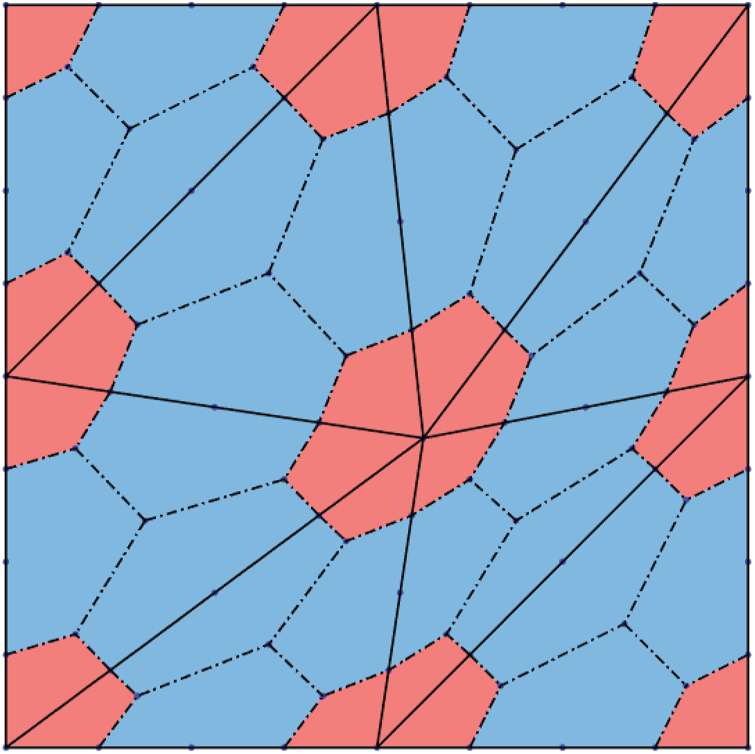
Figure 1: The primary mesh and dual mesh

In order to define the test function space, we need to construct a dual mesh associated with 𝓒h, see the dashed line segments in Fig. 1. For any triangular element K=ΔP1P2P3 with P1=(x1,y1),P2=(x2,y2) and P3=(x3,y3), we denote the barycenter of K as Q, and the midpoints of the three sides as M1,M2 and M3, respectively, see Fig. 2. Gk,k+1 and Gk+1,k are the two points on PkPk+1, satisfying

|PkGk,k+1||PkPk+1|=|Gk+1,kPk+1||PkPk+1|=β1∈(0,12),(4)

while Pk,k+1 is a point on PkMk+1 such that

|PkPk,k+1||PkMk+1|=β2∈(0,23),(5)

where k is a periodic index with Period 3. Using the above notations, K can be further partitioned into six subcells, i.e., three quadrilaterals and three pentagons, see Fig. 2. Let 𝓝h be the set of all vertices and edge midpoints on the primary mesh 𝓒h. Then, KP*, the dual cell associated with P∈𝓝h, is defined as the union of the subcells sharing P, and the dual mesh is defined as 𝓒h*={KP*:∀P∈𝓝h}. Now, the test function space is chosen as

Vh={vh∈L2(Ω̄):vh∣KP*=constant,∀P∈𝓝h∘;vh∣KP*=0,∀P∈𝓝h∩∂Ω}, where 𝓝h∘=𝓝h\∂Ω. Here we remark that the dual mesh 𝓒h* and the test function space Vh depend on two parameters β1 and β2. Different choices of the pair (β1,β2) lead to different finite volume element schemes.

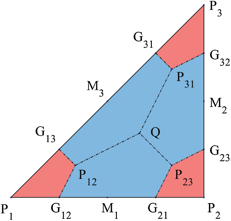
Figure 2: Partition of the triangular element K

2.2 Semi-Discrete Schemes

In this part, we propose the following spatial discrete formulation of Eq. (1), ∫Ω(∂u∂t-∂αΔu∂tα-Δu)vhdxdy=∫Ω(f(u)+g)vhdxdy,∀vh∈Vh.

By the divergence theorem and the definition of Vh, we have,

∫KP*∂u∂tdxdy-∫∂KP*(∂α∇u∂tα⋅nP*+∇u⋅nP*)ds=∫KP*(f(u)+g)dxdy,∀P∈𝓝h∘,(6)

where ∇ is the gradient operator and nP* is the unit normal vector outward to ∂KP*. The left hand-side of Eq. (6) can be rewritten as

∫KP*∂u∂tdxdy-∫∂KP*(∂α∇u∂tα⋅nP*+∇u⋅nP*)ds=∑K∈𝓒h[∫KP∂u∂tdxdy-∫εK,P(∂α∇u∂tα+∇u)ds⋅nP*], where KP=K⋂ KP* and εK,P=K⋂ ∂KP*. Based on the above formulation, we formulate the semi-discrete finite volume element solution of the Eq. (6) as: Find uh=uh(x,y,t)∈Uh with t∈(0,T], such that

∑K∈𝓒h[∫KP∂uh∂tdxdy-∫εK,P(∂α∇uh∂tα+∇uh)ds⋅nP*]=∑K∈𝓒h∫KP(f(uh)+g)dxdy,∀P∈𝓝h∘.(7)

For the computation of the terms in Eq. (7), we introduce the following affine mapping that transforms K onto K^ in (λ1,λ2) plane,

{λ1=1JK(|y21y31|x-|x21x31|y+|x2y2x3y3|),λ2=1JK(|y31y11|x-|x31x11|y+|x3y3x1y1|),(8)

where

JK=|x1y11x2y21x3y31|, and K^ is the reference element whose vertices and barycenter are specified by P^1=(1,0),P^2=(0,1),P^3=(0,0) and Q^=(1/3,1/3), respectively, see Fig. 3. Let uh,K be the restriction of uh on K. Then, under the affine mapping Eq. (8), the counterparts of uh and uh,K can be expressed as ûh=ûh(λ1,λ2,t),ûh,K^=∑j=16uj,Kϕ^j(λ1,λ2), where uj,K=uh(Pj),uj+3,K=uh(Mj),j=1,2,3,

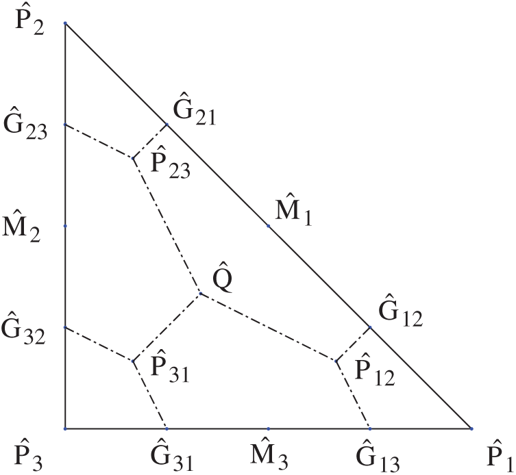
Figure 3: The reference element K^ and its associated subcells

ϕ^j(λ1,λ2)(1≤j≤6) are the shape functions on K^, given by

{ϕ^1(λ1,λ2)=λ1(2λ1-1),ϕ^2(λ1,λ2)=λ2(2λ2-1),ϕ^3(λ1,λ2)=λ3(2λ3-1),ϕ^4(λ1,λ2)=4λ1λ2,ϕ^5(λ1,λ2)=4λ2λ3,ϕ^6(λ1,λ2)=4λ1λ3, and λ3=1-λ1-λ2. Now we rewrite Eq. (7) to get the following semi-discrete schemes,

∑K∈𝓒h[∫K^P∂ûh∂tJKdλ1dλ2-∫ε^K,P(∂α∇ûh∂tα+∇ûh)FK,Pdl⋅nP*]=∑K∈𝓒h∫K^P(f(ûh)+ĝ)JKdλ1dλ2,(9)

where P∈𝓝h∘ and FK,P denotes the ratio of the measures of εK,P and ε^K,P. One can see that ∇ûh,K^=∑j=16uj,K∇ϕ^j, where

∇ϕ^j=(∂ϕ^j∂x∂ϕ^j∂y)=(∂ϕ^j∂λ1∂λ1∂x+∂ϕ^j∂λ2∂λ2∂x∂ϕ^j∂λ1∂λ1∂y+∂ϕ^j∂λ2∂λ2∂y)=(∂λ1∂x∂λ2∂x∂λ1∂y∂λ2∂y)∇^ϕ^j, and ∇^ is the gradient operator with respect to (λ1,λ2) plane. By straightforward calculations, we have ∇^ϕ^1=(4λ1-10),∇^ϕ^2=(04λ2-1),∇^ϕ^3=(4λ1+4λ2-34λ1+4λ2-3),∇^ϕ^4=4(λ2λ1),∇^ϕ^5=4(-λ2-λ1-2λ2+1),∇^ϕ^6=4(-2λ1-λ2+1-λ1).

2.3 Fully Discrete Schemes

Next we introduce the fully discrete schemes at time tn-α/2. Let 0=t0<t1<⋯<tN=T be a uniform partition of the time interval [0,T] with mesh length Δt=T/N, and tn=nΔt (n=0,1,2,…,N). For any function z(t), let zn = z(tn).

Lemma 2.1. ([14], Lemma 2) Suppose z(t)∈C3[0,T]. Then, we have

∂z∂t(tn-α2)={1Δt(z1-z0)+𝓞(Δt),n=1,12Δt[(3-α)zn-(4-2α)zn-1+(1-α)zn-2]+𝓞(Δt2),n≥2.(10)

Lemma 2.2. ([11], Lemma 2) Assume that f(t)∈C2[0,T]. Then, the following second-order formula for the approximation of the nonlinear term at time tn-α/2 holds,

f(z(tn-α2))=(2-α2)f(zn-1)-(1-α2)f(zn-2)+𝓞(Δt2),n≥2.(11)

Lemma 2.3. ([15], Lemma 2) Suppose z(t)∈C3[0,T]. We have the following L2-1σ formula at time tn-α/2,

∂αz∂tα(tn-α2)=Δt-αΓ(2-α)[c0nzn-∑j=1n-1(cn-j-1n-cn-jn)zj-cn-1nz0]+𝓞(Δt3-α),(12)

where c01=a0, for n = 1, and for n≥2,

cln={a0+b1,l=0,al+bl+1-bl,1≤l≤n-2,al-bl,l=n-1, with a0=(1-α2)1-α,al=(l+1-α2)1-α-(l-α2)1-α,l≥1,bl=12-α[(l+1-α2)2-α-(l-α2)2-α]-12[(l+1-α2)1-α+(l-α2)1-α],l≥1.

Based on Lemmas 2.1–2.3, we propose the following fully discrete schemes by the Eq. (9) at time tn-α/2:

for n = 1,

∑K∈Th{ ∫K^P1Δt(u^h1−u^h0)JKdλ1dλ2−∫ε^K,P[ c01Δt−αΓ(2−α)(∇u^h1−∇u^h0)+((1−α2)∇u^h1+α2∇u^h0) ]FK,Pdl⋅nP* } =∑K∈Th∫K^P(f(u^h0)+g^1−α2)JKdλ1dλ2, ∀P∈Nh°;(13)

for n≥2,

∑K∈Th{∫K^P12Δt((3−α)u^hn−(4−2α)u^hn−1+(1−α)u^hn−2)JKdλ1dλ2 −∫ε^K,P[ Δt−αΓ(2−α)(c0n∇u^hn−∑j=1n−1(cn−j−1n−cn−jn)∇u^hj−cn−1n∇u^h0)+((1−α2)∇u^hn+α2∇u^hn−1) ] ×FK, Pdl⋅nP*}=∑K∈Th∫K^P[ ((2−α2)f(u^hn−1)−(1−α2)f(u^hn−2))+g^n−α2 ]JKdλ1dλ2, ∀P∈Nh°,(14)

where ûhn=ûhn(λ1,λ2,tn), n=0,1,…,N.

Let the basis functions of the trial function space Uh be denoted as φk(x,y), (k=1,2,…,m) where m is the number of unknowns (i.e., m=#𝓝h∘), then the numerical solution uhn=(φ1,φ2,…,φm)⋅uhn∈Uh, where the vector uhn=(u1n,u2n,…,umn)T, (n=0,1,…,N). Moreover, we know ûhn=(φ^1,φ^2,…,φ^m)⋅uhn, where φ^k(λ1,λ2), (k=1,2,…,m) are transformed from φk(x,y), (k=1,2,…,m) by the affine mapping Eq. (8). By simplifying and synthesizing the Eqs. (13), (14), we obtain the following matrix form of the fully discrete schemes:

for n = 1,

Muh1-[c01Δt1-αΓ(2-α)+Δt(1-α2)]Auh1=ΔtMf0+Δtg1-α2+Muh0-c01Δt1-αΓ(2-α)Auh0+Δtα2Auh0;(15)

for n≥2,

(3−α)Muhn−[ 2c0nΔt1−αΓ(2−α)+2Δt(1−α2) ]Auhn=2ΔtM[ (2−α2)fn−1−(1−α2)f n−2 ]+2Δtgn−α2 +(4−2α)Muhn−1−(1−α)Muhn−2−2Δt1−αΓ(2−α)A[ ∑j=1n−1(cn−j−1n−cn−jn)uhj+cn−1nuh0 ]+ΔtαAuhn−1,(16)

where

fn=(fkn)m×1, fkn=f(uhn(Pk)), Pk∈Nh°, (17)

gn−α2=(gkn−α2)m×1, gkn−α2=∑K∈Th∫K^Pkg^n−α2JKdλ1dλ2, Pk∈Nh°, (18)

mass matrix M=∑K∈𝓒hMK and stiffness matrix A=∑K∈𝓒hAK. Meanwhile, MK and AK, square matrices of degree m, are expanded by the element matrices MK and AK as follows:

MK=(mij)6×6, mij=∫K^Piϕ^jJKdλ1dλ2, (19)

AK=(aij)6×6, aij=∫ε^K,Pi∇ϕ^jFK, Pdl⋅nPi*, (20)

where KPi=K⋂ KPi* and εK,Pi=K⋂ ∂KPi* are transformed to K^Pi and ε^K,Pi by the affine mapping Eq. (8) and Pi (i=1,…,6) (Pj+3=Mj,j=1,2,3) are vertices or edge midpoints of the element K.

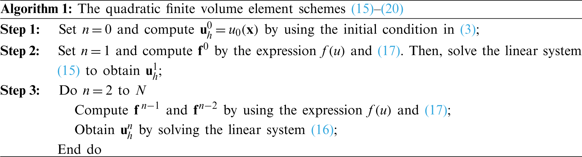
For the above finite volume element schemes, we emphasize that the nonlinear term is approximated by using the linearized difference scheme in Lemma 2.2, and none nonlinear iteration is involved. The whole algorithm is summarized below.

3  Numerical Examples

In this section, we use Eqs. (15)–(20) to solve four examples on uniform triangular mesh (Mesh I) and random triangular mesh (Mesh II), respectively, see Figs. 4, 5. The first level of Mesh II is constructed from Mesh I by the following random distortion of the interior vertices,

x:=x+ωηxh,y:=y+ωηyh, where ω∈(0,0.5) is the disturbance coefficient, h is the spatial mesh size, ηx and ηy are two random numbers located in [-1,1]. The subsequent level is refined by the standard bisection procedure from its previous level. In our numerical examples, we choose the disturbance coefficient ω=0.2 for Mesh II (see Fig. 5). Recall that our quadratic finite volume element schemes have two parameters β1 and β2. Here we just investigate the following specific schemes:

•   First scheme (QFVE-1): β1=(3-3)/6, β2=(6+3-21+63)/9;

•   Second scheme (QFVE-2): β1=β2=(3-3)/6;

•   Third scheme (QFVE-3): β1=1/4, β2=1/3;

•   Fourth scheme (QFVE-4): β1=β2=1/3.

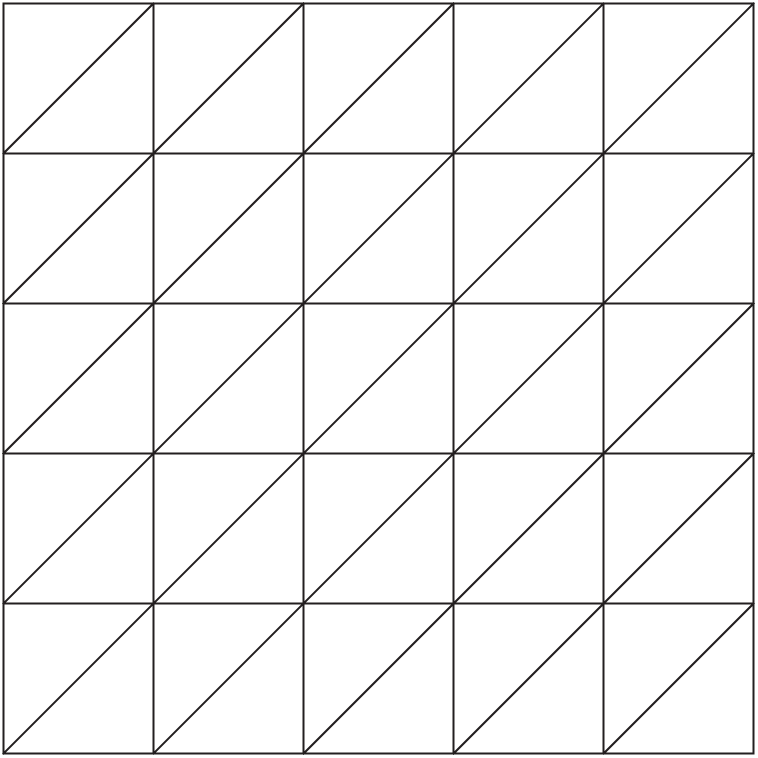
Figure 4: Uniform triangular mesh (Mesh I)

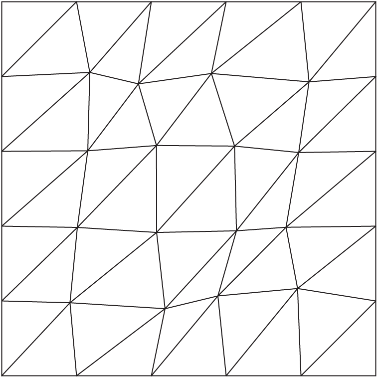
Figure 5: Random triangular mesh (Mesh II)

We remark that the counterparts of the above schemes for elliptic problems have been studied in [42,43,46,47], respectively. The L2 errors Eu and convergence orders Ru1, Ru2 are defined as Eu= max1≤n≤N(∑K∈𝓒h∫K(uh(x,y,tn)-u(x,y,tn))2dxdy)12,Ru1=log(Eu(h2)/Eu(h1))log(h2/h1),Ru2=log(Eu(Δt2)/Eu(Δt1))log(Δt2/Δt1), respectively, where h1 and h2 are the spatial mesh sizes of two successive meshes, and Δt1 and Δt2 are the mesh sizes of two successive time levels. Moreover, the results of the quadratic finite element scheme (QFE) [29] are also employed for comparison.

3.1 Example 1

Solve Eqs. (1)–(3) with the nonlinear term f(u) = u2 and the source term g(x,t)=[(3+α)t2+α+8π2t3+α+4π2t33Γ(4+α)]sin(2πx)sin(2πy)-t6+2α sin2(2πx)sin2(2πy), where Ω̄=[0,1]2 and T = 1. The exact solution is u(x,t)=t3+α sin(2πx)sin(2πy). We choose Δt=1/2000, h = 1/10 and α=0.1. Fig. 6 shows the exact solution u and the vertex values of the numerical solution uh at x = 0.3 and t = 1 on Mesh I, which implies that the numerical solution can well approximate the exact solution even though the five schemes exhibit difference in accuracy. Tabs. 1, 2 gives some detailed results for the quadratic finite volume element schemes and quadratic finite element scheme. In Figs. 7, 8, we draw log-log plots of the L2 errors vs. with mesh size h on Mesh I and Mesh II when Δt=1/2000. One can see that spatial convergence orders of the QFE and QFVE-1 schemes are close to 3 for different α, while the spatial convergence order of other quadratic finite volume element schemes (QFVE-2, QFVE-3, QFVE-4) are nearly 2 and lower than that of QFVE-1, which agrees with the observations made in [49] for elliptic problems. Moreover, we calculate temporal convergence orders of these schemes in Tabs. 3, 4, and we can find the temporal convergence orders are nearly 2.

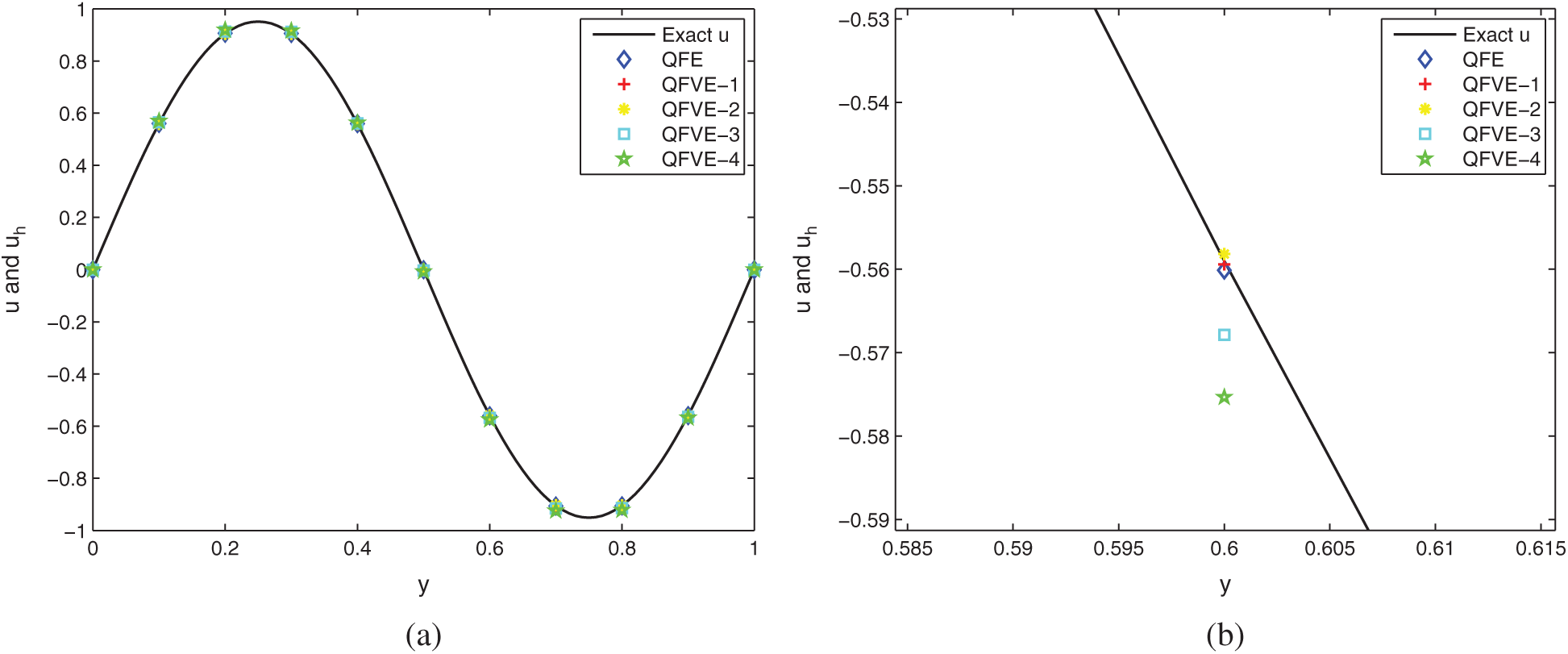
Figure 6: Comparison of the numerical solutions and the exact solution for Example 1 on Mesh I. (a) A full profile; (b) A local enlarged profile

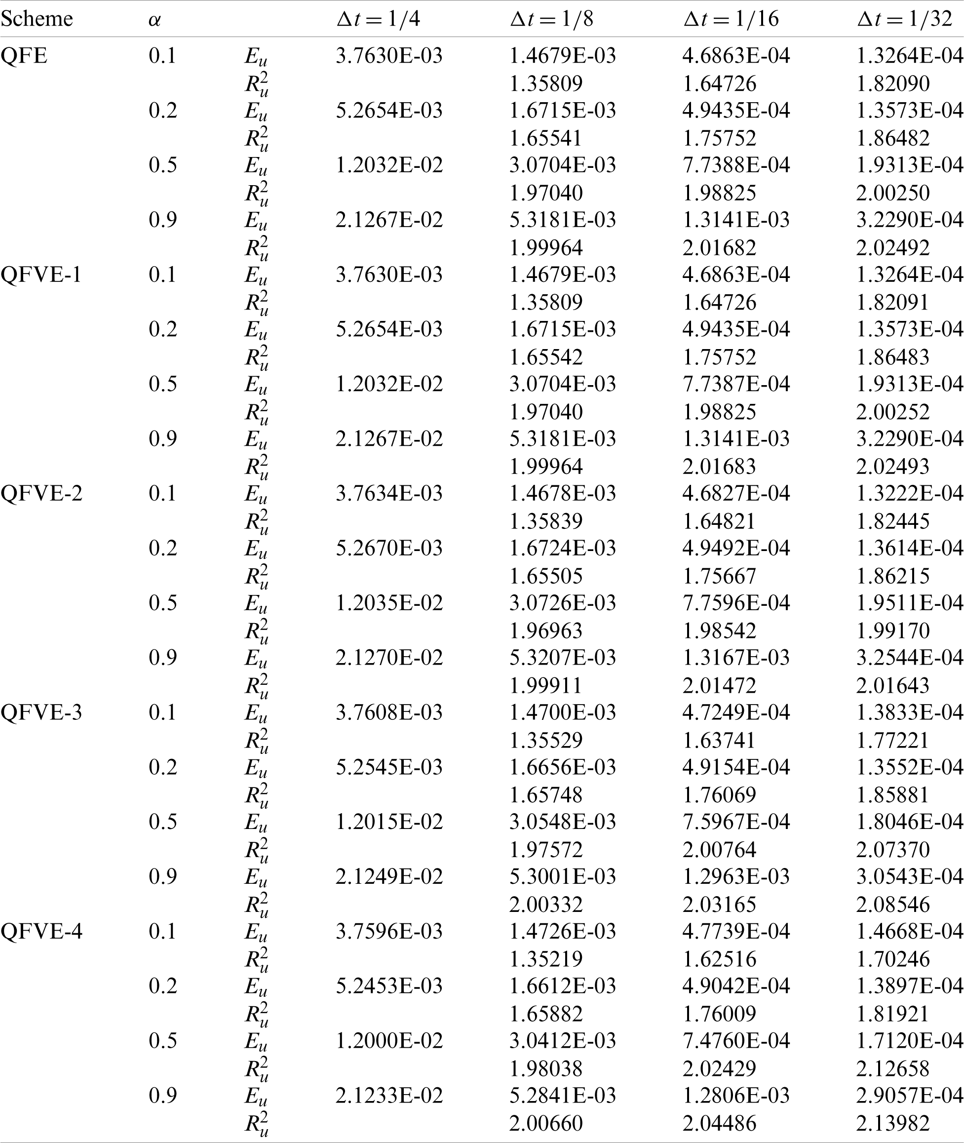
Table 1: Error results and spatial convergence orders with Δt=1/2000 on Mesh I in Example 1

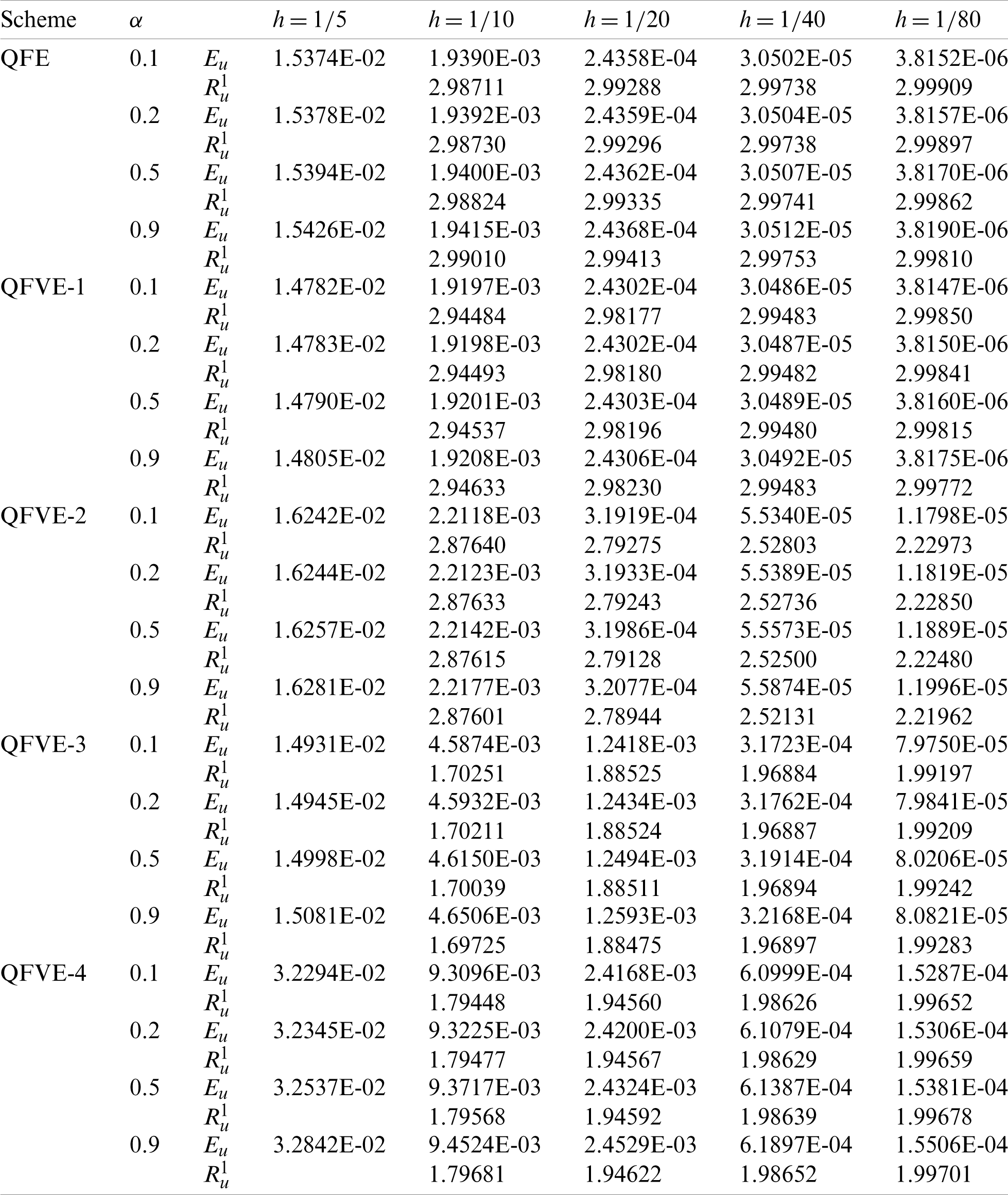
Table 2: Error results and spatial convergence orders with Δt=1/2000 on Mesh II in Example 1

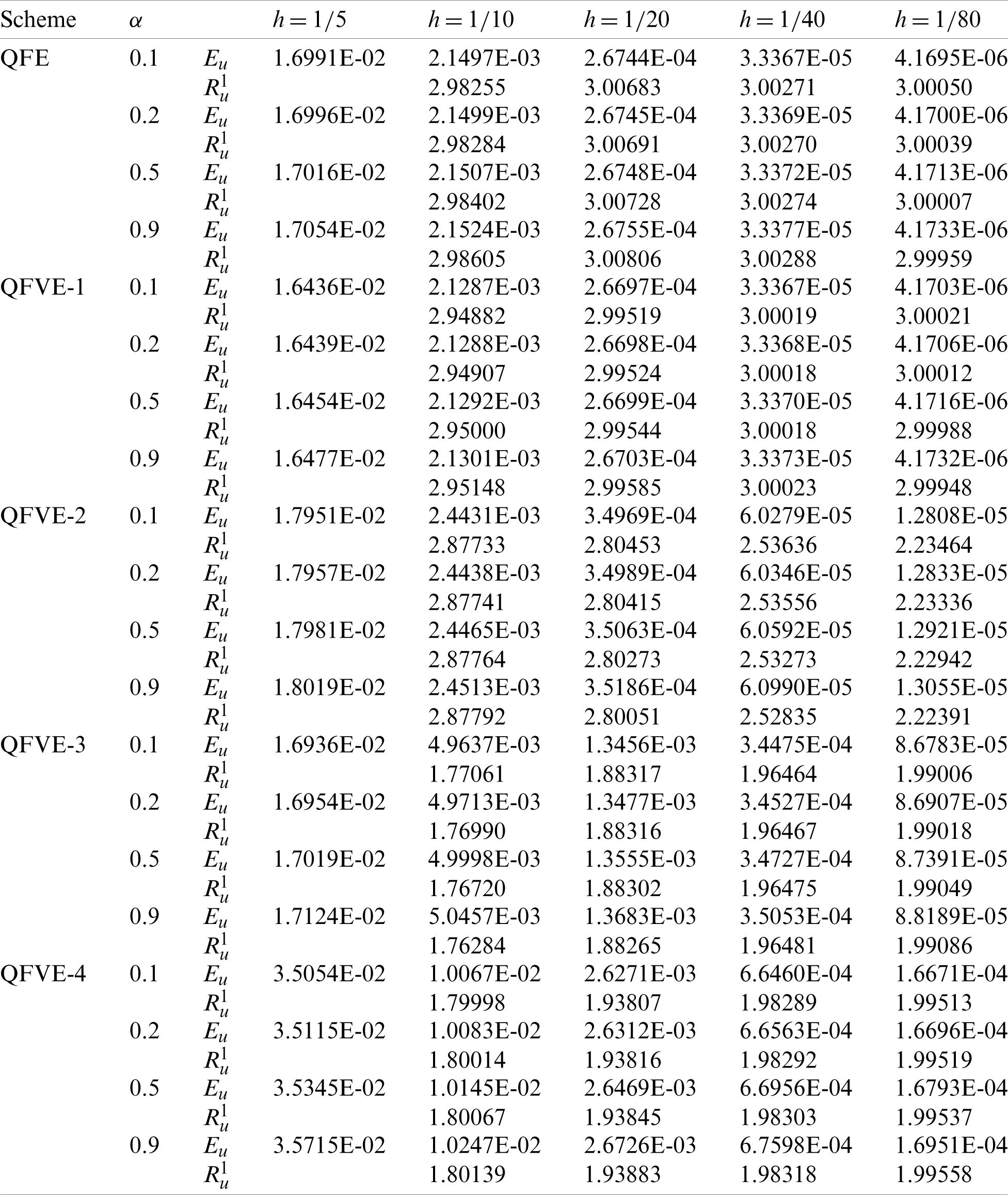
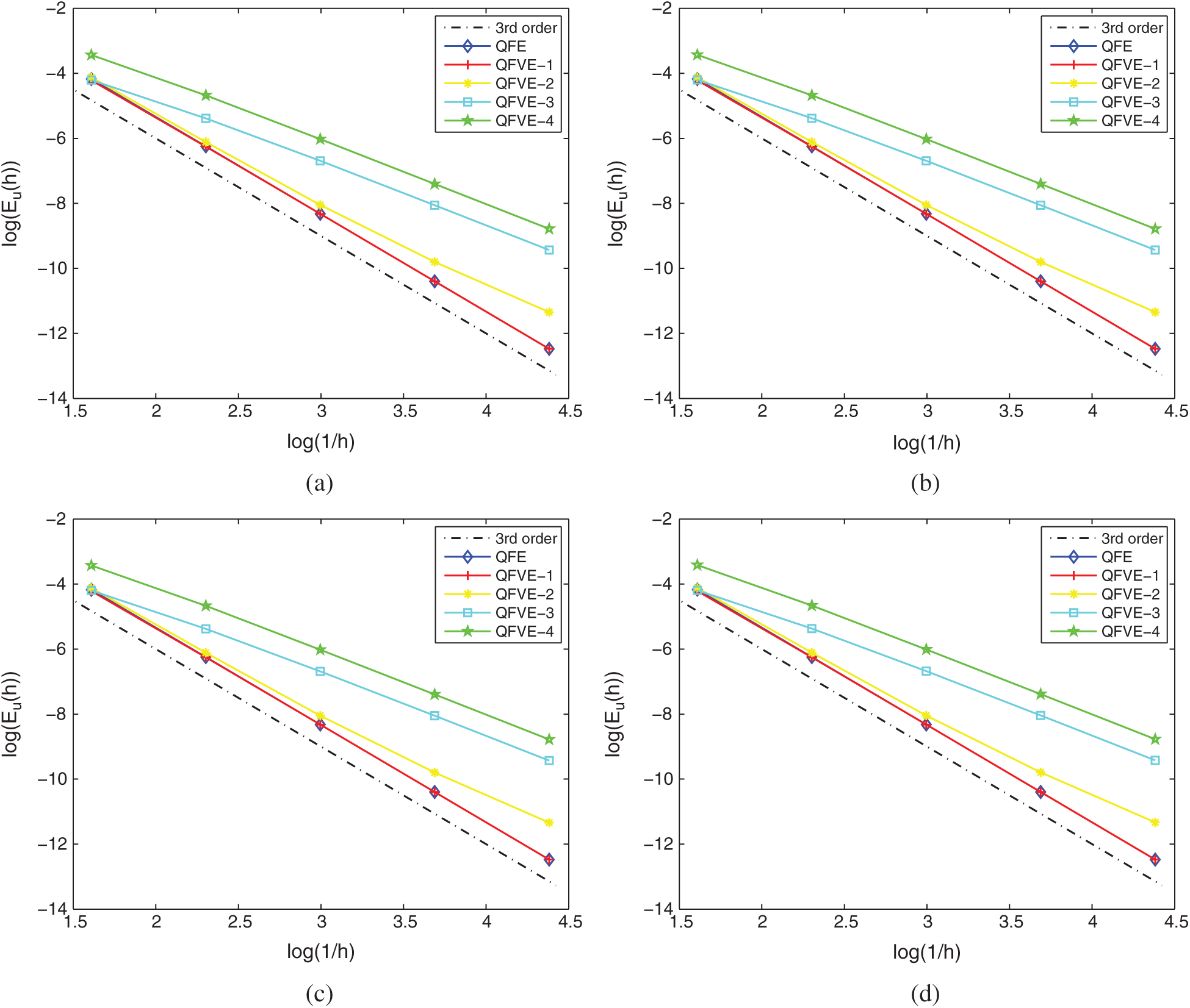
Figure 7: L2 errors of the numerical solution on Mesh I in Example 1. (a) α=0.1; (b) α=0.2; (c) α=0.5; (d) α=0.9

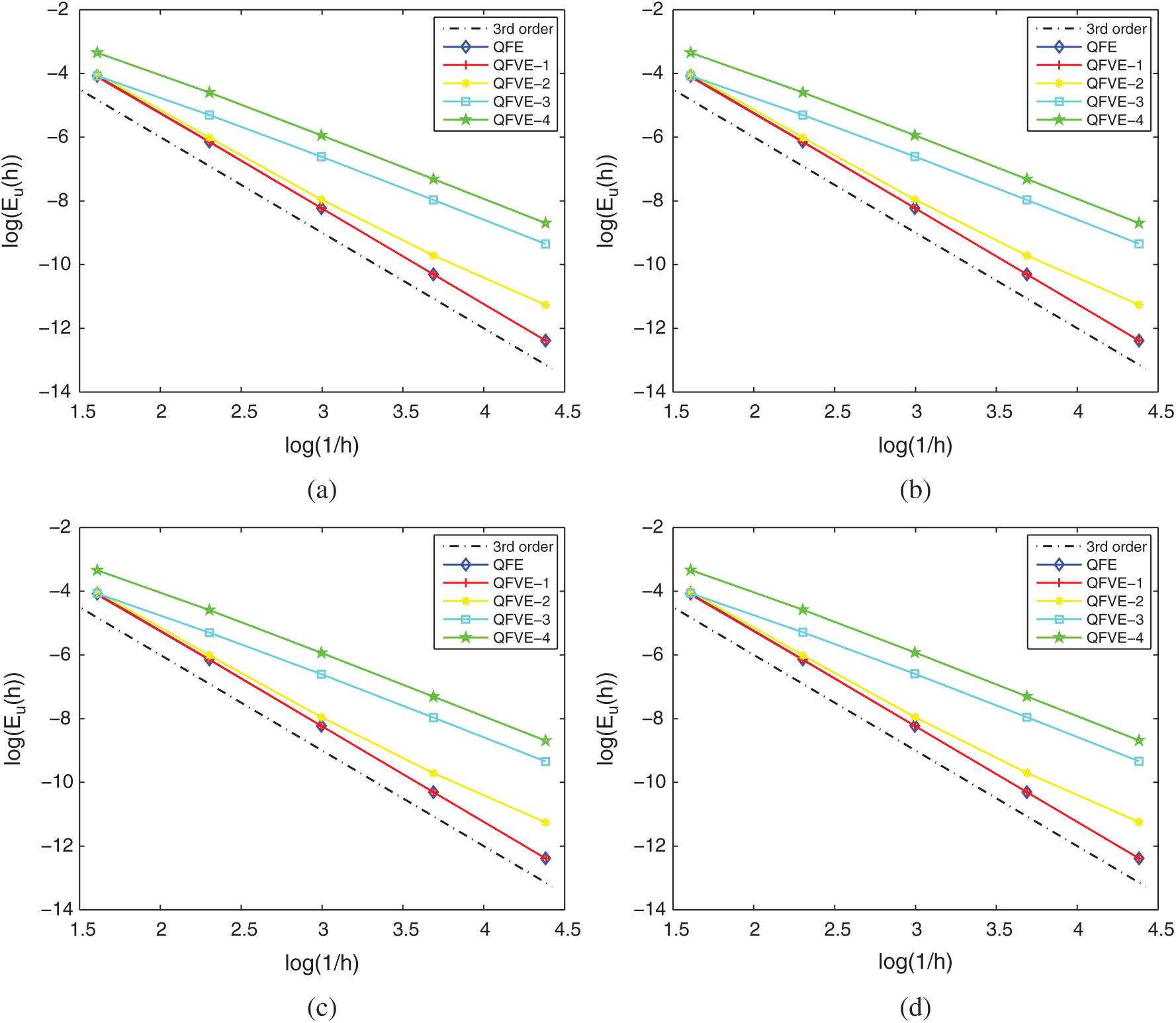
Figure 8: L2 errors of the numerical solution on Mesh II in Example 1. (a) α=0.1; (b) α=0.2; (c) α=0.5; (d) α=0.9

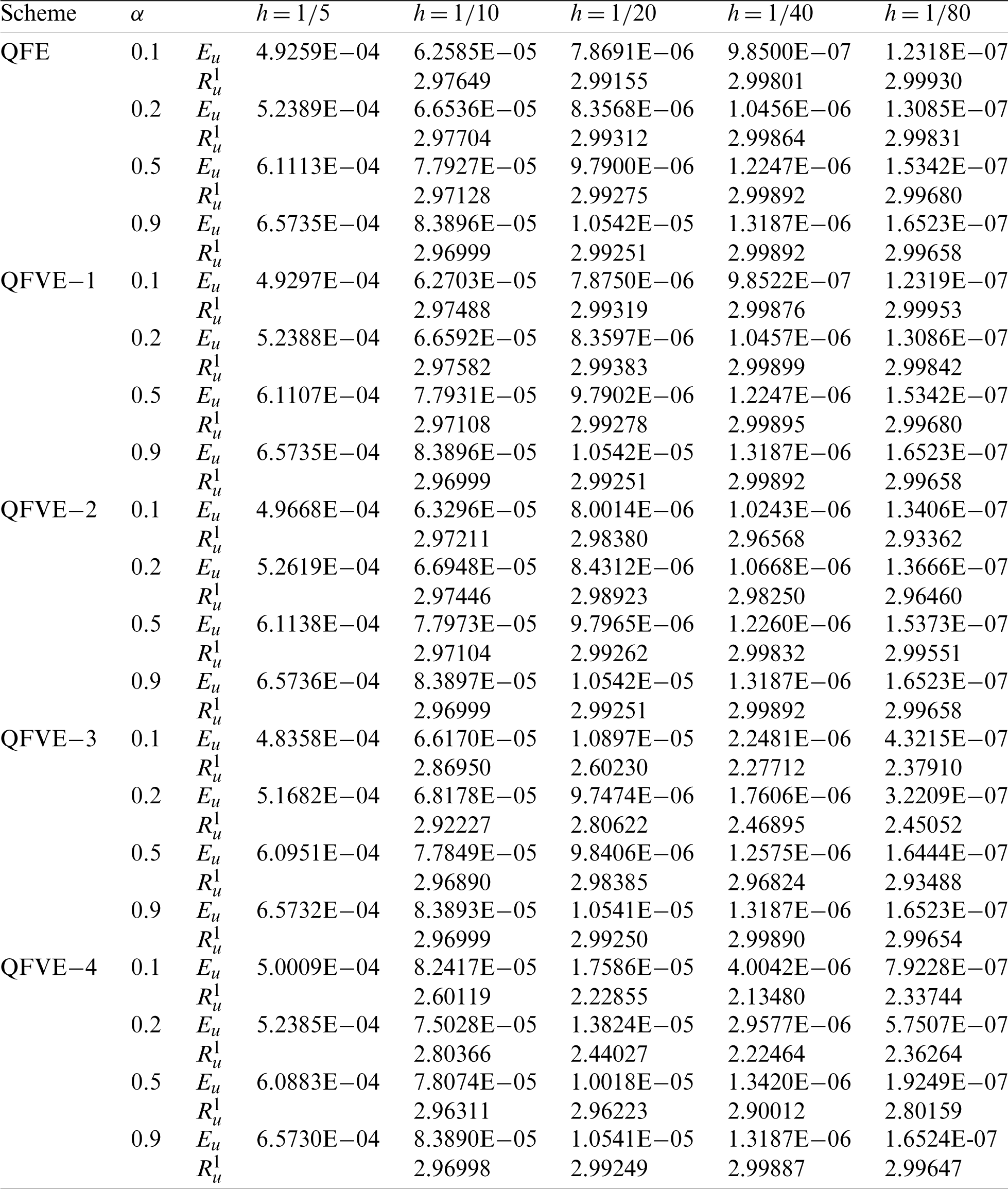
Table 3: Error results and temporal convergence orders with h = 1/160 on Mesh I in Example 1

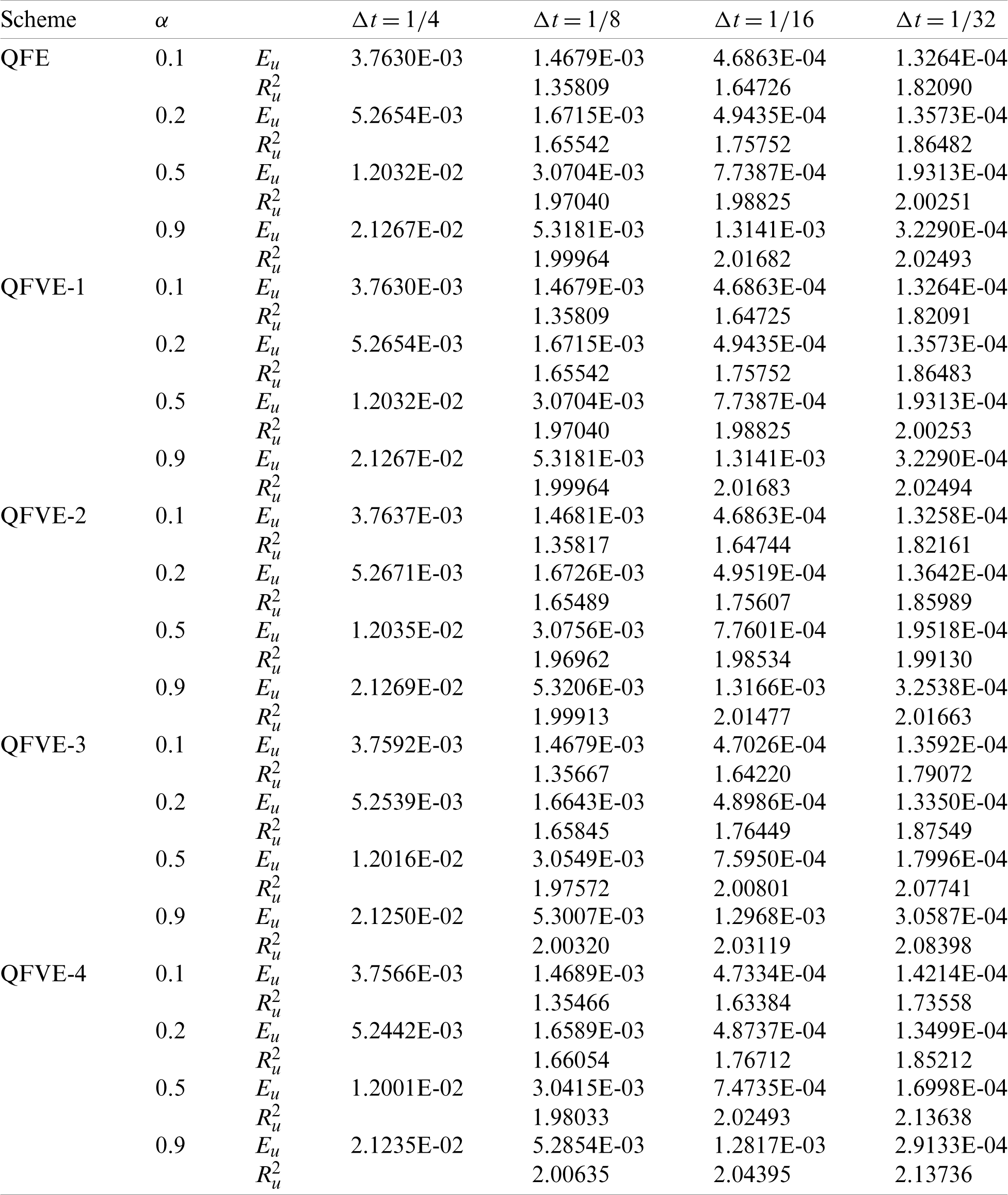
Table 4: Error results and temporal convergence orders with h = 1/160 on Mesh II in Example 1

3.2 Example 2

Solve Eqs. (1)–(3) with Ω̄=[0,2]2, T = 2, f(u)= sin(u) and g(x,t)=3t2g1(x)-12[t3+6t3-αΓ(4-α)]g2(x)- sin(t3g1(x)), where g1(x)=x(x-0.5)(x-1.5)(x-2)y(y-0.5)(y-1.5)(y-2), g2(x)=x(x-0.5)(x-1.5)(x-2)(y2-2y+1924)+y(y-0.5)(y-1.5)(y-2)(x2-2x+1924).

Table 5: Error results and spatial convergence orders with Δt=1/2000 on Mesh I in Example 2

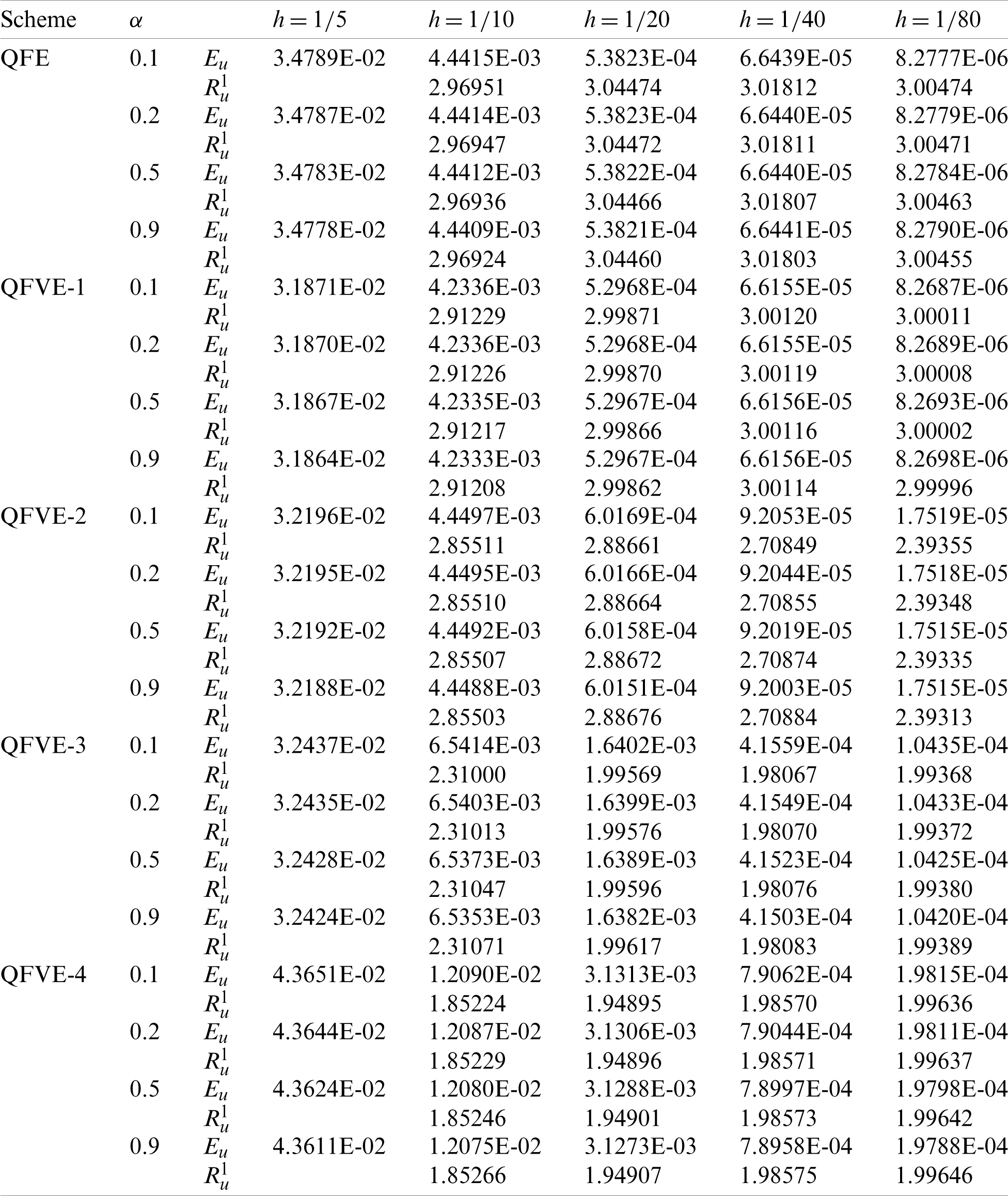
Table 6: Error results and spatial convergence orders with Δt=1/2000 on Mesh II in Example 2

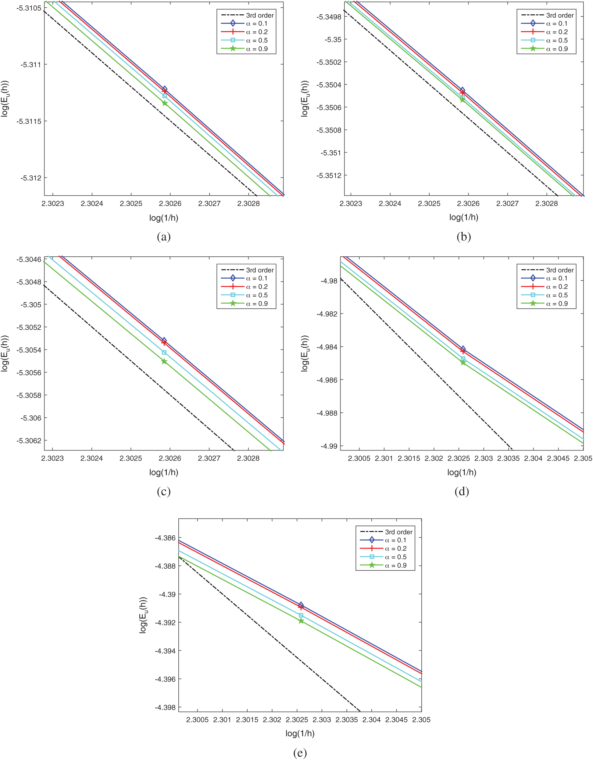
Figure 9: L2 errors of the numerical solution on Mesh II in Example 2. (a) QFE; (b) QFVE-1; (c) QFVE-2; (d) QFVE-3; (e) QFVE-4

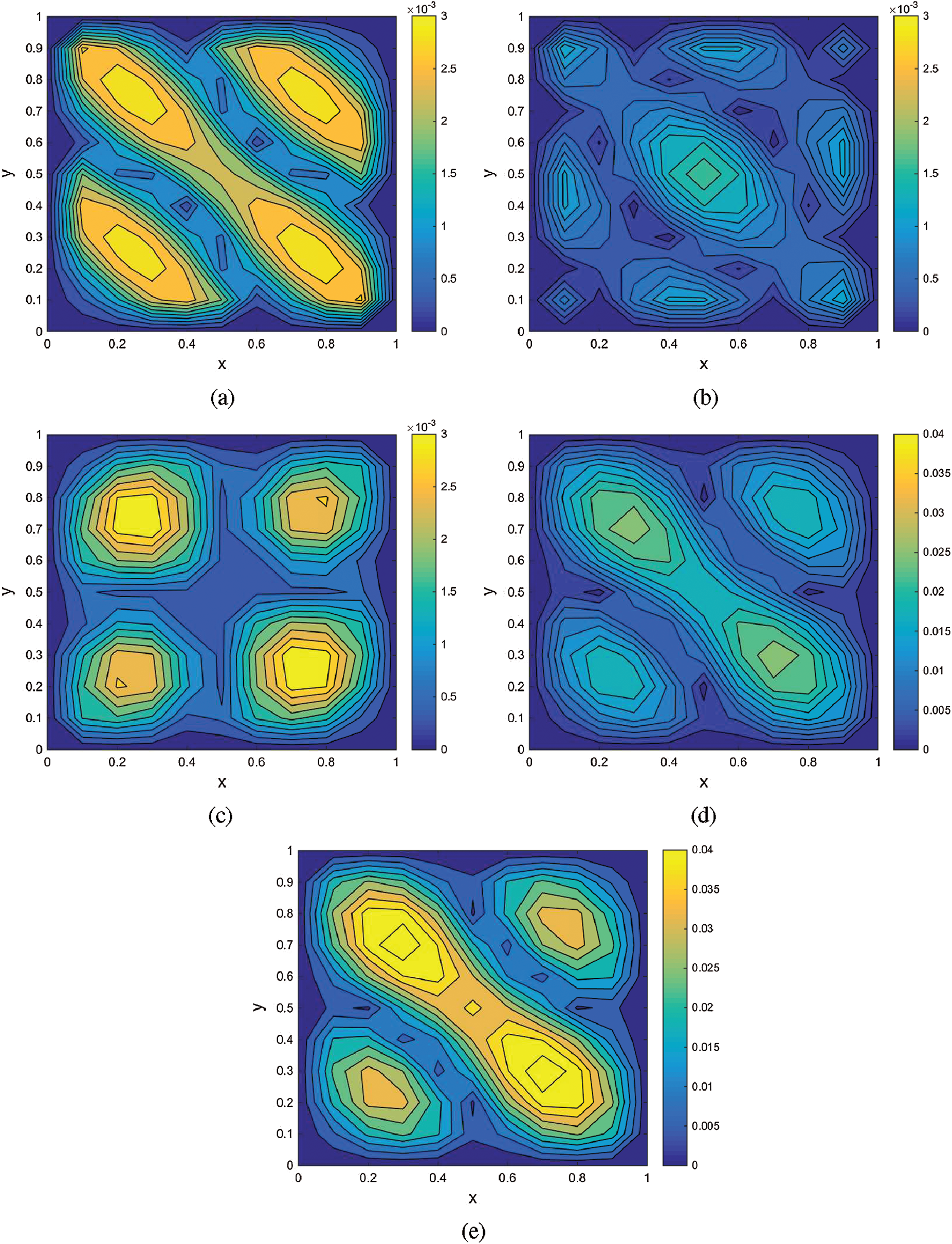
Figure 10: Contour plots of |u − uh| on Mesh I in Example 3. (a) QFE; (b) QFVE-1; (c) QFVE-2; (d) QFVE-3; (e) QFVE-4

Table 7: Numerical results with Δt=1/2000 on Mesh I in Example 3

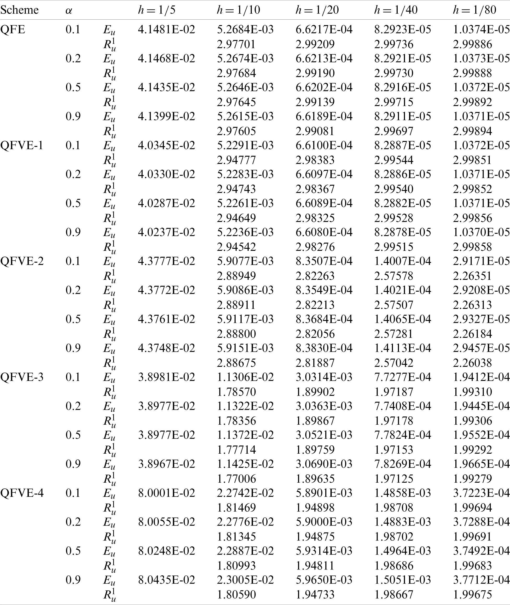
Table 8: Numerical results with Δt=1/2000 on Mesh II in Example 3

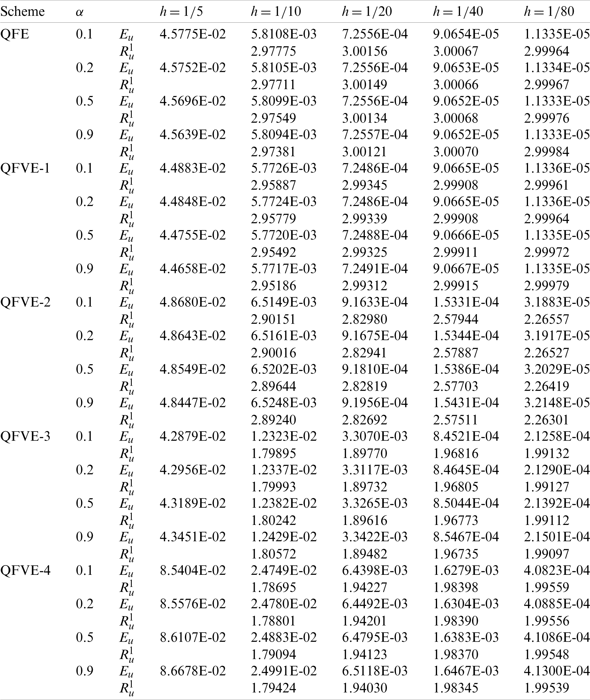
Table 9: Numerical results with Δt=1/100 on Mesh I in Example 4

The exact solution to this example is:

u(x,t)=t3x(x-0.5)(x-1.5)(x-2)y(y-0.5)(y-1.5)(y-2).

Analogously, we calculate the L2 errors and spatial convergence orders for several kinds of quadratic finite volume element schemes and quadratic finite element scheme, see Tabs. 5, 6. The convergence behavior is similar to that for Example 1. Moreover, when α=0.1, 0.2, 0.5, 0.9 we draw the log–log plots for these five schemes on Mesh II, and find that the converge orders don’t change with α, see Fig. 9.

3.3 Example 3

We take the space-time domain Ω̄×[0,T]=[0,1]2×[0,1], the nonlinear term f(u) = u3 − u and the source term

g(x,t)=[2et+8π2et+8π2t1-αE1,2-α(t)]sin(2πx)sin(2πy)-e3t sin3(2πx)sin3(2πy), where Mittag–Leffler function E1,2-α(t) is defined by E1,2-α(t)=∑i=0∞tiΓ(i+2-α).