Engineering & Sciences
| Computer Modeling in Engineering & Sciences |
DOI: 10.32604/cmes.2021.014119
ARTICLE
Classification of Domestic Refuse in Medical Institutions Based on Transfer Learning and Convolutional Neural Network
1School of Control Engineering, Chengdu University of Information Technology, Chengdu, 610225, China
2College of Automation, Chongqing University of Posts and Telecommunications, Chongqing, 400065, China
3Department of Informatics, University of Leicester, Leicester, LE1 7RH, UK
*Corresponding Author: Hanbing Yan. Email: yanhb@cuit.edu.cn
Received: 01 September 2020; Accepted: 01 February 2021
Abstract: The problem of domestic refuse is becoming more and more serious with the use of all kinds of equipment in medical institutions. This matter arouses people’s attention. Traditional artificial waste classification is subjective and cannot be put accurately; moreover, the working environment of sorting is poor and the efficiency is low. Therefore, automated and effective sorting is needed. In view of the current development of deep learning, it can provide a good auxiliary role for classification and realize automatic classification. In this paper, the ResNet-50 convolutional neural network based on the transfer learning method is applied to design the image classifier to obtain the domestic refuse classification with high accuracy. By comparing the method designed in this paper with back propagation neural network and convolutional neural network, it is concluded that the CNN based on transfer learning method applied in this paper with higher accuracy rate and lower false detection rate. Further, under the shortage situation of data samples, the method with transfer learning and ResNet-50 training model is effective to improve the accuracy of image classification.
Keywords: Domestic refuse; image classification deep learning; transfer learning; convolutional neural network
Faced with the situation of increasing domestic refuse in medical institutions output and deteriorating environmental conditions, how to utilize waste resources and improve the quality of living environment through garbage classification management is one of the urgent issues for all countries in the world. Medical waste management is of great importance due to its infectious and hazardous nature that can cause undesirable effects on humans and the environment [1]. The work with good garbage classification, can not only save resources, reduce environmental pollution and land occupation, but also for the sake of human health, social sustainable development. At present, many countries are starting to concern the garbage classification. The errors in garbage classification will cause the overall unsatisfactory result, which requires to arrange manpower to classify secondly. However, the working environment of this traditional garbage classification method is poor and the sorting efficiency is low. These results suggest that the quantities of medical waste are not controlled, and hospitals have a defective monitoring management system of their waste [2]. Song et al. [3] analyzed the harm of medical waste and composition, especially, pointed out the importance of medical waste management, such as the awareness of the harm, medical waste sorting, and some effective monitoring mechanisms. Medical waste is related with our health, environment, economic and society. Therefore, more delicate measures are needed in collection, storage, transfer and disposal of medical waste.
With the development of image recognition technology, image classification based on machine learning involves all aspects of human life. At present, image classification technology has been widely used to detect and identify various objects. In the field of medicine [4], due to the intuitive, non-invasive, safe and convenient characteristics, image recognition technology is widely applied in clinical diagnosis and pathological research to help complete automatic recognition of medical image diagnosis, digitize auxiliary medical diagnosis process, and reduce the workload of medical workers. In terms of crop disease prevention [5], the convolutional neural network (CNN) is used to automatically identify rice sheath blight, one of the three major diseases affecting rice production and planting, to make up for the lack of artificial judgment, which is conducive to the accurate identification and prevention of rice sheath blight. A deep learning CNN was applied to classify the type of e-waste, and a faster region-based convolutional neural network (R-CNN) was used to detect the category and size of the waste equipment in the images [6]. The development of machine learning technology is gradually becoming mature, which can be fully used to realize the extraction and classification of garbage image features. Under the condition of ensuring the classification speed and accuracy, the cost of labor and time can be saved. It will contribute to the improvement of their knowledge of medical waste classification.
If the machine learning techniques are used to implement medical waste classification, it will improve the scientific awareness of garbage classification and garbage sorting efficiency. This paper is based on deep learning technology in machine learning methods, and designs an image classifier. By using deep learning method of neural network algorithm, it realizes garbage classification with high precision, high efficiency. The work of proper waste separation will greatly alleviate the environmental pollution caused by wrong garbage classification.
The organization of this paper is as follows. In Section 2, related works are briefly reviewed. In Section 3, The main algorithms are introduced, it includes the BP neural network, ResNet-50 convolutional neural network and ResNet-50 convolutional neural network based on the transfer learning method. Section 4 describes the good performance in quality and quantitative experimental results for the proposed algorithm. Finally, conclusions are drawn in Section 5.
In view of the research on garbage image classification methods, Cai et al. [7] added color classification of plastic garbage on the basis of waste plastic garbage classification with materials in 2007. The color space features of different waste plastics were extracted. The color space patterns based on I1, I2 and I3 were selected. Back propagation (BP) neural network was used for pattern recognition of various colors. It realized the classification of waste plastics. In 2016, Mittal et al. [8] initialized the parameters of the target neural network with the pre-training model of AlexNet convolutional neural network [9], and took the GINI data set as the training set of garbage image classification model. After 150,000 iterations of training, the accuracy of the final model in garbage image recognition reached 87.69%. 2018, Rabano et al. [10] used MobileNet deep learning and transfer learning with the aid of model parameters in ImageNet large visual recognition challenge data set. It included common garbage classification training: glass, paper, cardboard, plastic, metal and other waste. After 500 iterations training, it finally got spam image classifier testing accuracy with 87.2%. In 2019, Zhao et al. [11] used different wavelengths of light reflectance spectrum information from garbage, through the establishment of classification model and analyze the reflectivity spectrum information, finally realized garbage image recognition and classification. In 2020, Yuan et al. [12] applied a 23-layer convolutional neural network model to garbage classification. It emphasized on the real-time garbage classification and solved the low accuracy of garbage classification. In the same year, Lu et al. [13] also used convolutional neural network iteration to train a classifier model for garbage classification.
Some machine learning, vision algorithms and fusion methods are employed in the garbage sorting. For example, Chen et al. [14] proposed a vision-based robotic grasping system by deep learning for garbage sorting, with region proposal generation and the modified VGG-16 model. They proposed an intelligent garbage classifier with identification method, efficient separation system and intelligent control system by variety of sensors and machine vision technology [15]. Cao et al. [16] proposed a method of garbage classification and recognition by transfer learning, which migrated the existing InceptionV3 model recognition on the dataset to identify garbage, with the training accuracy 99.3% and the test accuracy 93.2%, respectively. Ma et al. [17] proposed an enhanced single shot multibox detector with a lightweight and novel feature fusion module to solve the problems of heavy tasks and low sorting efficiency in garbage sorting with mean average precision 83.48%. They proposed an architecture to classify waste videos through features learnt by 2D convolutional and 3D convolutional neural networks. In their paper, the accuracy is 79.99% in the challenging dataset [18].
The application of neural network in garbage classifier is more and more popular, because it overcomes the limitation on the input dimension of BP neural network. In the framework of neural network, the image can be directly as input data. Due to the weights of the shared characteristics in convolution the training of the neural network, it can save much time. For traditional machine learning, a large number of training samples are needed to extract effective image features and achieve the required accuracy. It is not easy to collect certain types of images in some classification problems, because sufficient training data cannot be guaranteed. This will lead to the failure of classification accuracy, what’s more, a large number of image feature extraction will consume a great amount of training time cost.
To solve these problems, transfer learning method is adopted, which transfers the parameters of the pre-training model after a large number of sample training to the model used for training classifier. Since it already contains enough feature parameters for image classification, the neural network parameter only needs to fine-tune the final full connection layer, according to the number of classification categories. When the classifier model is generated, it is only necessary to train the final full connection layer and fix the weight of transferred parameters. The transfer learning method not only shorts training time, but also ensures the high accuracy of image classification.
The selection of neural network determines the quality of image feature extraction and the accuracy of classification. In this paper, BP neural network, ResNet-50 convolutional neural network and ResNet-50 convolutional neural network combining with transfer learning are discussed respectively. By verifying the training and verification sets of the same training set, the neural network with the best classification effect is selected to generate the final classifier model.
Neural network is a network with multiple levels and feedback systems, which is divided into the following three layers: input layer, hidden layer and output layer [19]. The neurons are transmitted layer by layer. If there is an error between the output and the ideal value, the back propagation is carried out. In the process of error back propagation, the weight and threshold of the network are adjusted by the gradient of error change [20]. After each iteration training, the difference between the predicted results obtained by BP neural network and the real value will gradually decrease.
In 1986, Rumelhart et al. [21] proposed error back propagation neural network (BP network). The network is a multi-layer forward network of one-way propagation. The BP algorithm of error back propagation is called BP algorithm and its basic idea is gradient descent method. The gradient search technique is used to minimize the mean square error between the actual output value and the expected output value. ui is the internal state of the neuron,
Generally, from Eq. (1),
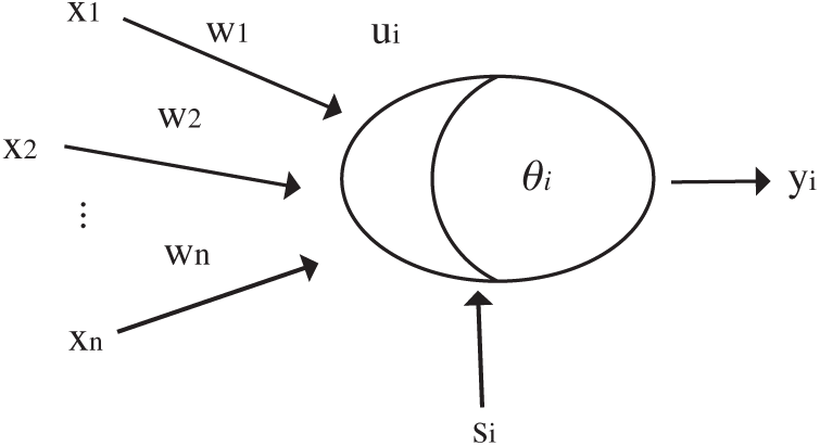
Figure 1: Neuronal structural model
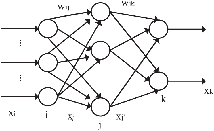
Figure 2: BP neural network structure
3.2 Convolutional Neural Network
CNN is a kind of feedforward neural network, which is composed of input layer, convolution layer, pooling layer, activation layer, full connection layer and output layer [22]. Unlike BP neural network, images can be directly used as input data to the convolutional neural network. The output of the convolutional neural network is converted into the relative probability of categories through Softmax [23], and the category with the highest probability is taken as the final classification result. After feature extraction in the convolutional layer, the output feature map [24] will be transferred to the pooling layer for feature selection and information filtering. Because the number of feature maps are determined by the convolution kernel, the dimension of feature maps obtained by convolution operation is very large, which will lead to increase computation cost and the computing burden of computer equipment.
The activation layer [25] can carry out nonlinear mapping for the output of the convolutional layer. The Sigmoid and ReLU functions are commonly used in neural networks. ReLU function is commonly used in convolutional neural networks, because Sigmoid function is used to calculate the error gradient in back propagation, which requires a relatively large amount of computation. Moreover, gradient explosion is likely to occur in back propagation with deep networks. The output layer of the convolutional neural network is the probability of converting the output of the full connection layer into each type through the Softmax function. The Softmax function is shown in Eq. (2):
where Zi is the output value of the full connection layer,and Si is the probability value of the i class.
To express quantitative differences in neural network calculation results and the actual category, the output of the Softmax is combined with the actual category labels to construct cross entropy model, calculation formula is shown in Eq. (3), N is the number the training in the batch sample, C is the classification number,
The parameter matrix of the convolutional neural network is updated by using the weight of the loss function and the gradient of the offset. For example, a weight matrix W with
According to the partial derivatives of the weight matrix of the loss function in Eq. (3), parameters are updated to form a new weight matrix W′ :
The weights and bias of convolution neural network in the training process is similar to the BP neural network. Both include the loss function and the actual values of gradient parameters, which are considered as the basis of updating parameters and the overall gradient is in a downward trend. The convolutional neural network model parameters are adjusted to image classification task and achieve the goal of classification accuracy.
3.2.1 ResNet-50 Convolutional Neural Network
As the number of layers increases in the convolutional neural network, gradient dissipation and gradient explosion are likely to result in the decrease of accuracy of the training model. ResNet [26] are applied the residual structure to solve this problem, which can ensure that the performance of the network can be improved with the augment of the depth of the neural network. Fig. 3 is the structure diagram of residual block.
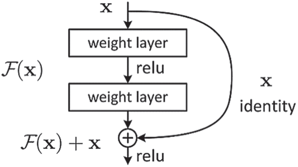
Figure 3: Structure diagram of residual block
ResNet is with two mapping relationships: Identity mapping and residual mapping. The final residual block structure output is shown in Eq. (6), where x is identity mapping, and the residual mapping is
From Eq. (6), the residual block of the original input is added directly to the original positive propagation path. When the gradient is obtained by BP neural network, due to the existence of x, gradient
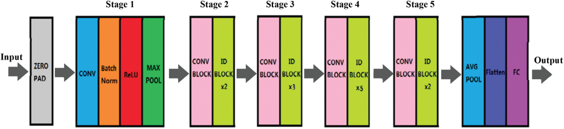
Figure 4: ResNet-50 structure chart
From stages 2 to 5,
3.2.2 Based on Transfer Learning ResNet-50 Convolutional Neural Network
Transfer learning [29] is one method of the machine learning, which can reuse the model parameters developed for one task in another different task and serve as the starting point of another task model. This is a common approach in deep learning. In terms of computer vision and natural language processing, the development of neural network model requires a large amount of computing and time resources, and the technical span is also large. Therefore, the parameters of the pre-training model are often reused as starting points for computer vision and natural language processing tasks. The central idea of transfer learning is in Fig. 5.
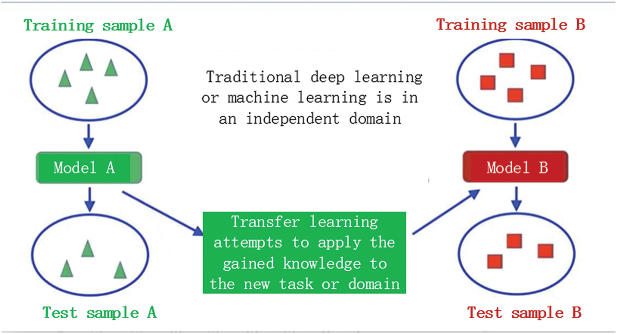
Figure 5: The central idea of transfer learning
Transfer learning takes the model developed for task A as the starting point and reuses it in the process of developing the model for task B. The main advantage of transfer learning is that it saves training time and, in most cases, the neural network can achieve better performance without a lot of data. Transfer learning is employed in these situations, for example, the current task lacks training data. There are already neural network learners trained with a large amount of data in the approximate field. Fig. 6 lists two strategies for transfer learning, these are: finetuning, freeze and train. Finetuning includes the pre-training network on the underlying data set and training all layers in the target data set. Freeze and train include freezing all layers except the last layer (weights are not updated) and training the last layer. You can also freeze the first few layers and fine-tune the rest.
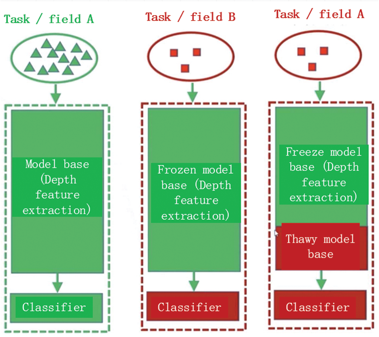
Figure 6: Two strategies for transfer learning
The transfer learning is often used in the following scenario. Firstly, Small target set, image similarity: When the target data set is smaller than the basic data set and the image is similar, it is recommended to freeze and train, and only train the last layer. Secondly, Large target set, image similarity: Fine tuning is recommended. Thirdly, Small target set, different images: It is recommended to take freezing and training, training the last layer or the last layer. Fourthly, Large target set with different images: fine tuning is recommended.
In the application of image classification, traditional machine learning algorithms require sufficient image data as training samples, some of which are difficult to obtain. With the increasing number of neural network layers, it will take a lot of time to update the parameters of each layer through training. If the whole neural network is retrained, it will consume a lot of time and labor cost. The transfer learning approach can overcome these difficulties. The features of the underlying image extracted from the pre-trained convolutional neural network model are universal in many classification problems, and the classification accuracy can be higher even with fewer training samples. The ResNet-50 convolutional neural network based on transfer learning combines the advantages of transfer learning and ResNet residual structure, which can ensure high classification accuracy on the basis of reducing training time.
4.1 Data Set Collection and Image Preprocessing
According to management measures on garbage classification [30], garbage is divided into the following four categories: other garbage, perishable garbage, recyclable garbage and hazardous garbage. The range of Sigmoid function is [0, 1]. Medical waste refers to waste with direct or indirect infectivity, toxicity and other hazards produced by medical and health institutions in medical treatment, prevention, health care and other related activities. Whether the management of medical waste can achieve standardized management is a major concern of the current society. The effective management of medical waste is an important way and link to control the spread of the epidemic and an effective measure to prevent and control environmental pollution and harm to human survival [31]. According to the circular, the household waste generated in medical institutions can be classified into four categories: hazardous waste (labeled by waste 3), recyclable waste (labeled by waste 2), perishable waste (labeled by waste 1) and other waste (labeled by waste 0). Hazardous waste mainly includes waste batteries, waste fluorescent tubes, waste film and waste paper. This category also consists of harmful and highly polluting substances, such as medicine box, drug bag, infusion tube, needle tube. Recyclable materials mainly include infusion bottles (bags) that have not been contaminated by patients’ blood, body fluids and excreta, plastic packaging bags, packaging boxes, paper packaging, express package, washbasin, clothes rack, empty beverage bottle, waste electrical and electronic products, and discarded hospital beds, wheelchairs, infusion racks, etc., after being wiped or fumigated. Perishable garbage mainly includes kitchen garbage, melon and fruit garbage, flower garbage, dishes, cigarette end, eggshell, and so on generated in the canteen, office building and other areas. In the data-set, other waste is what we don’t know the name of the garbage generally and it is infrequent relatively in our life.
For the above four types of sample data, the number of each type of data is 2000, which is divided into a training set of 1600 and a verification set of 400. As the input of neural network, the garbage images need preprocessing to meet the input requirements of the algorithm. At the same time, image preprocessing can improve the training speed and classification accuracy of neural network. The steps of image preprocessing are as follows:
The size of the input image of ResNet-50 convolutional neural network model is specified as
4.2 Confounding Matrix and Model Evaluation
Confounding matrix [33] is mainly used to compare the classification results with the actual measured values, and it will show the accuracy of the classification results. The columns of the confounding matrix represent the predicted categories, and the rows represent the actual categories. The values on the diagonal of the confounding matrix represent the correct part of the prediction, and the off-diagonal elements are the wrong part of the prediction. The higher the diagonal value is, the more correctly the prediction is. The evaluation of model classification mainly includes: accuracy rate and error detection rate [34]. positive (P) and negative (N) represent the judgment results of the model, and true (T) and false (F) evaluate whether the judgment results of the model are correct. For example, FP: the judgment of the model is positive, but the judgment result is actually wrong.
4.3 The Simulation of BP Neural Network Classifier
4.3.1 Determine the Number of Neurons in Each Layer and Hidden Layers
The size of the input image is
The neurons in the hidden layer are determined by empirical Eq. (7), where h is the number of nodes in the hidden layer, m is the number of nodes in the input layer, n is the number of nodes in the output layer, and a is the adjustment constant between 1 and 10.
Substitute the corresponding parameters into Eq. (7), and the number of hidden layer neurons in the experiment is 266.
4.3.2 Learning Rate and Batchsize Parameters
Parameter adjustment method: First, the batch size of each training is fixed, and the learning rate is set by 0.75, 0.075 and 0.0075 respectively, and the learning rate is iterated for 50 times to obtain the learning rate with the best convergence effect of the loss function. Then fix the optimal learning rate, set Batchsize of each training by 25, 50 and 75, respectively, and train iteration for 50 times to get the Batchsize with the best effect of loss function convergence.
It can be seen from Fig. 7 that too small a learning rate of 0.0075 leads to a slow convergence rate, while the learning rate of 0.75 is a fast convergence rate. It starts to oscillate and diverge after 10 iterations. Therefore, the learning rate is selected to be 0.075. Next, with fixed learning rate parameters, loss function reduction experiments with Batchsize 25, 50 and 75 are conducted, respectively.
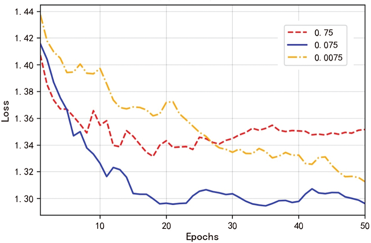
Figure 7: Comparison curve of loss reduction adjusted learning rate with Batchsize 50
In Fig. 8, the loss function curve with Batchsize 25 is the fastest and most stable decline. Combined with the above parameter adjustment experiment, BP neural network iterative training is conducted 100 times with the learning rate 0.075 and Batchsize 25. The trained model is used to classify the garbage image, and its confounding matrix is obtained as shown in Fig. 9.
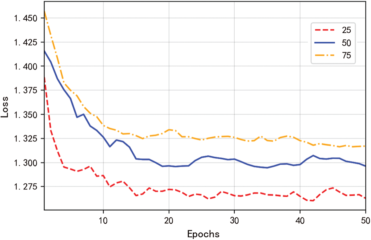
Figure 8: Comparison of loss reduction curves of adjusted Batchsize at learning rate 0.075
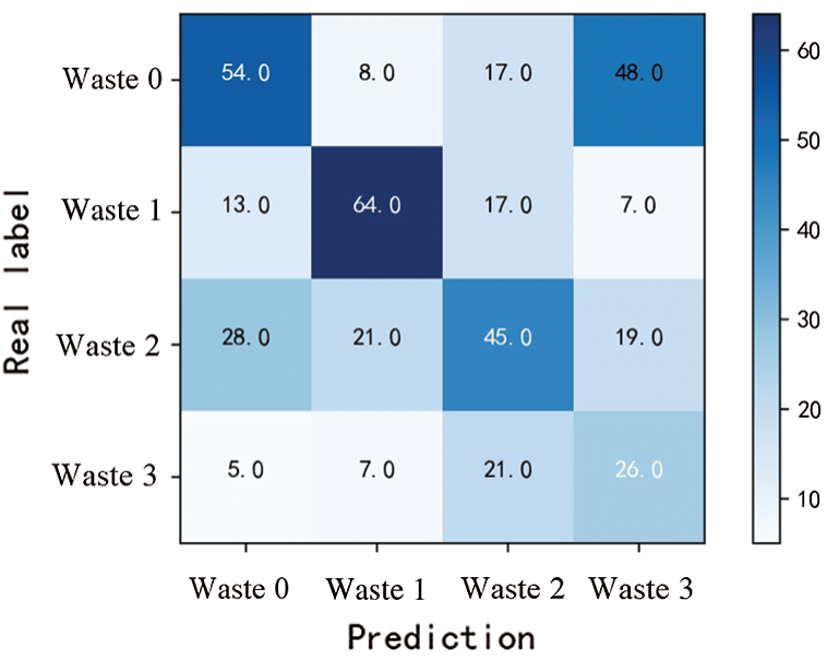
Figure 9: Confounding matrix of BP neural network
It can be seen from the confounding matrix of classification results of BP neural network in Fig. 9 that the classifier model trained by this method is the highest correct number of kitchen waste classification, with 64 frames. On the contrary, the correct amount of hazardous waste classification is the lowest, with 26 frames.
4.4 The Simulation of ResNet-50 Convolutional Neural Network Classifier
ResNet-50 convolutional neural network mainly conducts parameter tuning for learning rate parameter and Batchsize. In order to save parameter tuning time cost, the change value of learning rate is 0.5, 0.05 and 0.005, and the Batchsize 25, 50 and 75, respectively. In each case, 50 iterations of training are conducted. The loss function decline curve is obtained through iterative training, and the learning rate with the fastest convergence speed is selected. Then, the learning rate is fixed, and the Batchsize with the fastest convergence speed is also selected according to the loss function.
4.4.1 The Tuning of Earning Rate Parameter
The Batchsize of each training is fixed at 50, and the learning rate is set 0.5, 0.05 and 0.005, respectively. The learning rate of iterative training is performed 50 times, and the learning rate with the best effect of loss function convergence is obtained.
It can be seen from Fig. 10 that the learning rate 0.5 converges rapidly at the beginning, but the loss curve stops falling and even oscillates during the training. Learning rate 0.005 convergence rate is too slow, therefore, learning rate is selected 0.05.
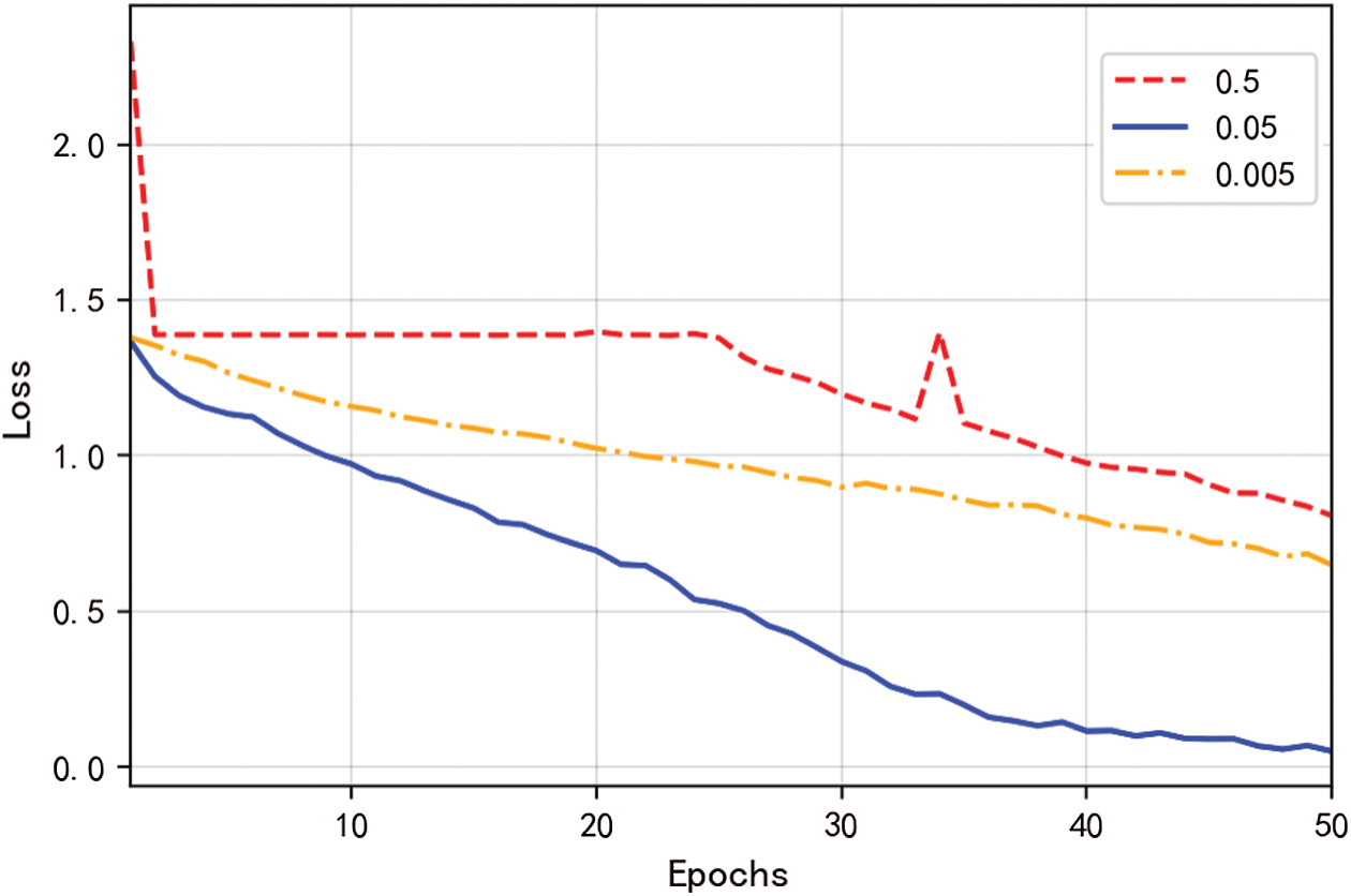
Figure 10: Comparison of learning rate loss decline curves with fixed Batchsize 50
4.4.2 The Tuning of Batchsize Parameter
Fix the optimal learning rate, set Batchsize of each training Batchsize by 25, 50, 75, and iterative training 50 times, and get the Batchsize with the best convergence effect of the loss function.
As can be seen from Fig. 11 that the Batchsize with the fastest convergence speed of the loss curve is 50. Combined with the above parameter adjustment experiment, the ResNet-50 convolutional neural network iterative training is conducted 100 times with the learning rate of 0.05 and Batchsize 50.
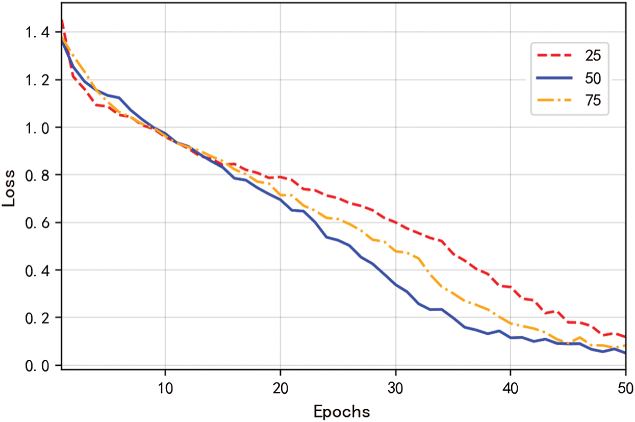
Figure 11: Comparison of Batchsize loss reduction curves with fixed learning rate 0.05
The trained model is used to classify the garbage image, and its confounding matrix is obtained as shown in Fig. 12.
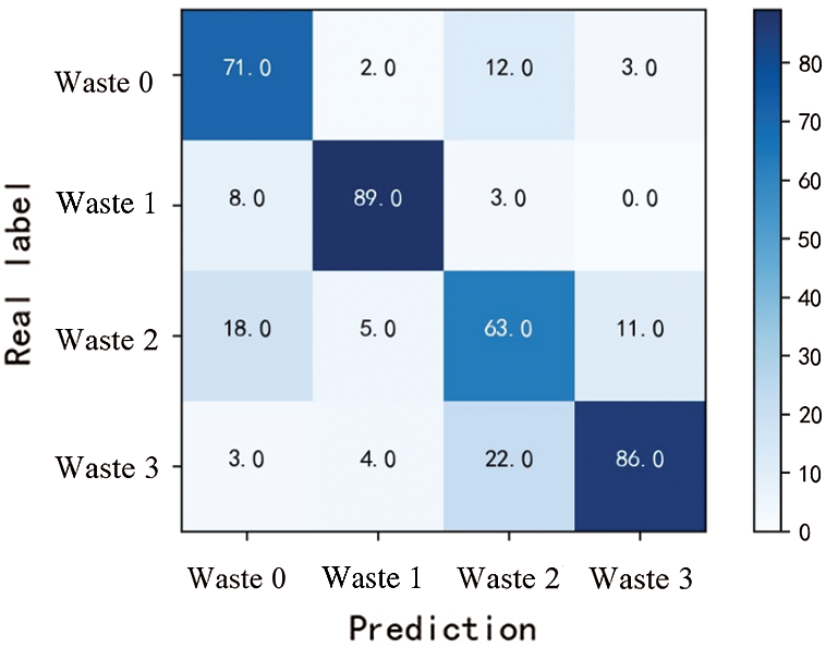
Figure 12: Confounding matrix of output results of RESnet-50 convolutional neural network
It can be seen that the confounding matrix of the classification results by ResNet-50 convolutional neural network in Fig. 12 that the classifier model trained by this method is the highest correct amount of waste classification with 89 frames. On the contrary, the number of hazardous wastes correctly classified is the lowest with a result of 63. As can be seen from the color depth of the heat map, the diagonal color is obviously compared with other positions, which indicates that ResNet-50 convolutional neural network is a high identification degree for these four types of garbage and is suitable for garbage image classification.
4.5 The Simulation of Resnet-50 Convolutional Neural Network Classifier and Transfer Learning
The ResNet-50 convolutional neural network parameter adjustment method based on transfer learning method is the same as ResNet-50 convolutional neural network, which also adjusts the learning rate and Batchsize parameters. The value of learning rate is selected 0.5, 0.05 and 0.005, and the Batchsize is 25, 50 and 75. 50 iteration training is conducted for each case. First, according to the decline of the loss function during iterative training, the learning rate with the fastest convergence speed is selected, then the learning rate is fixed, and the Batchsize with the fastest convergence speed is selected through the loss function.
4.5.1 The Tuning of Learning Rate Parameters
Fixed the Batchsize of each training, set the learning rate 0.5, 0.05 and 0.005, respectively, and conducted iterative training 50 times to obtain the learning rate with the best convergence effect of the loss function.
It can be seen from Fig. 13 that too small a learning rate 0.005 leads to a slow convergence rate, while the learning rate 0.5 will not decline after 3 iterations. Therefore, the learning rate is selected 0.05.
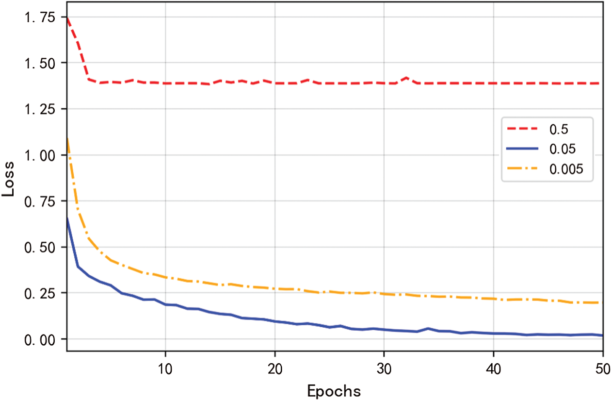
Figure 13: Comparison curve of loss reduction adjusted learning rate with fixed Batchsize 50
4.5.2 The Tuning of Batchsize Parameter
Fix the optimal learning rate and set Batchsize for each training 25, 50 and 75, respectively. After iterative training 50 times, the Batchsize with the best convergence effect of the loss function is obtained.
It can be seen in Fig. 14 that the loss function curve with Batchsize 50 is the fastest decreasing speed. Combined with the above parameter adjustment experiment, the ResNet-50 convolutional neural network iterative training is conducted 100 times with the learning rate 0.05 and Batchsize 50. The trained model is used to classify garbage images, and its confounding matrix is obtained as shown in Fig. 15.
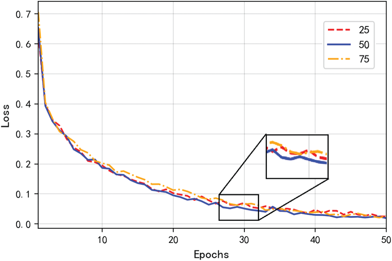
Figure 14: Comparison of loss reduction curves of Batchsize adjusted at a fixed learning rate 0.05
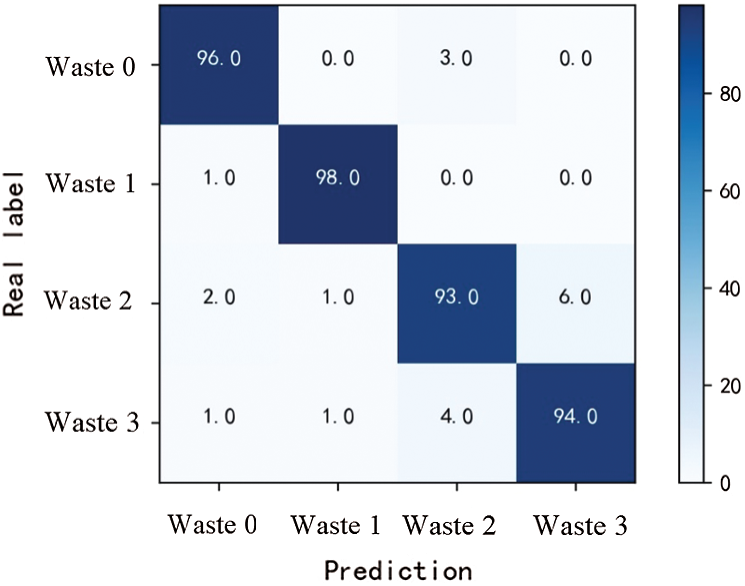
Figure 15: Confounding matrix of ResNet-50 convolutional neural network and transfer learning
It can be seen that the confounding matrix of the classification results of ResNet-50 convolutional neural network based on transfer learning in Fig. 15 that the classifier model trained by this method can correctly classify the four types of garbage with a quantity of more than 90 frames. The heat map corresponding to its confounding matrix is obvious diagonals, and the minimum number of correct classification is 93, which is higher than that of BP neural network and ResNet-50 convolutional neural network. The classifier obtained by ResNet-50 convolutional neural network training and transfer learning is a high identification degree for the types of garbage. This method combines the advantages of ResNet-50 convolutional neural network structure and transfer learning method, which not only ensures sufficient image feature extraction, but also saves the time of classifier training.
The BP neural network is with three layers, namely, the input layer, the hidden layer, and the output layer. This three-layer BP neural network can satisfy nonlinear mapping and is suitable for the training of medical waste image classifier. There is no standard library for medical waste classification yet. In this study, we use mobile phone shooting and web crawler to search and sort out the images, which are derived from actual images. The parameters are set as follows: iteration
The accuracy rate and average value of each method for different types of garbage are calculated by BP neural network, ResNet-50 convolutional neural network and ResNet-50 convolutional neural network based on transfer learning. Under the training of the same sample data, the ResNet-50 convolutional neural network based on transfer learning is the highest classification accuracy, with an average accuracy of 47.8% higher than that of BP neural network and 17.9% higher than that of ResNet-50 convolutional neural network without transfer learning. The bar diagram of accuracy comparison in the three methods is shown in Fig. 16.
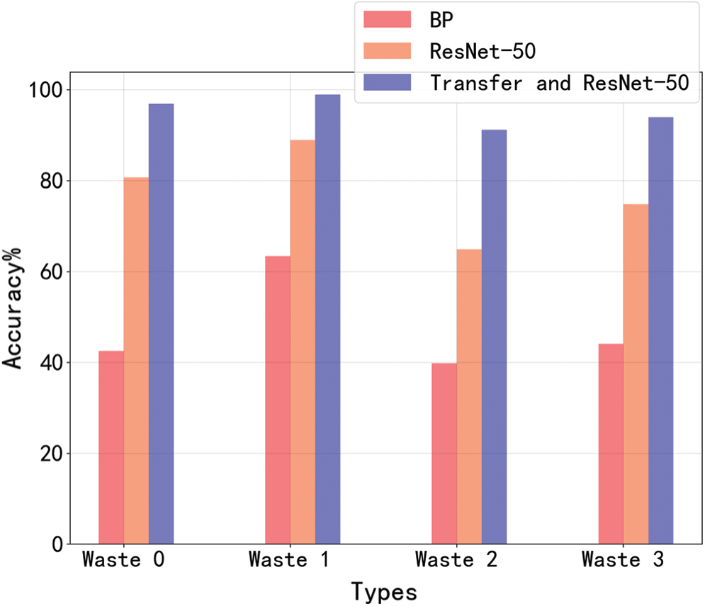
Figure 16: Accuracy comparison of bar chart
It can be seen from Fig. 16 that the classification accuracy of ResNet-50 convolutional neural network based on transfer learning is higher than that of BP neural network and ResNet-50 convolutional neural network for four different types of garbage. The classifier model trained in this method overcomes the problem that BP neural network cannot extract enough important features of the image, due to the limitation of the number of layers in the neural network, and also solves the problem that the classifier accuracy cannot be improved for the insufficient number of samples in ResNet-50 convolutional neural network.
4.6.2 Comparison of False Detection Rate
The error detection rate and average value of each method for different kinds of garbage are calculated. As can be seen from the classification results, under the training of the same sample data, the average false detection rate of ResNet-50 convolutional neural network and transfer learning is 16.0% lower than that of BP neural network and 5.9% lower than that of ResNet-50 convolutional neural network. The comparison diagram of the error detection rate of the three methods is shown in Fig. 17.
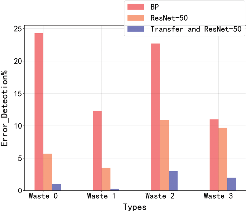
Figure 17: Comparison of error detection rate
From Fig. 17, the error detection rate of the classifier model obtained by ResNet-50 convolutional neural network training and transfer learning in four different types of garbage is much lower than that of BP neural network and ResNet-50 convolutional neural network. This method combines the advantages of transfer learning and ResNet-50 structure. It uses ResNet-50 pre-training model with rich sample features and residual structure to improve the identification degree of the classifier. It enhances the ability of classify in four kinds of garbage and effectively reduces the rate of false detection.
4.6.3 Object Classification Results
It can be seen from the classification results of the classifier that each frame (
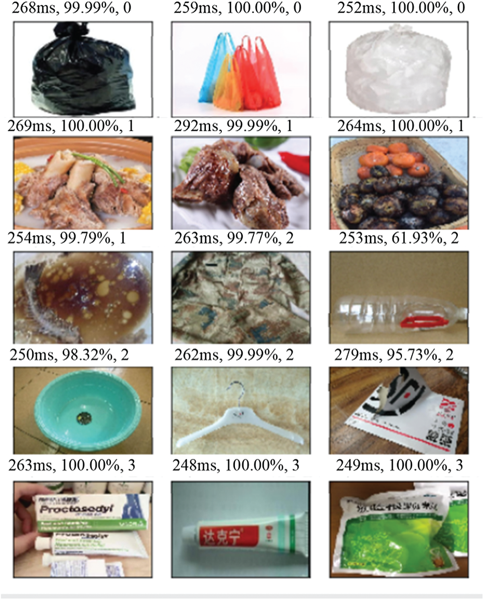
Figure 18: Results of classifier classification. The waste is classified into four categories: hazardous waste (labeled by waste 3), recyclable waste (labeled by waste 2), perishable garbage (labeled by waste 1) and other waste (labeled by waste 0)
4.6.4 Comparation with Other Waste Detection
To verify the effectiveness of our method, we select some representative algorithms for comparation. In the practical application, some garbage are linked with others, it is difficult to separate them into complete individual. The dataset is not exposed, and no standard datasets are found. Therefore, we used accuracy rates directly given in other authors’ papers for comparison.
From the quantity comparations in Tab. 1, the accuracy of our method is better than other results in the previous studies related to waste detection and classification. Our experimental results are better benefited from the employment of transfer learning, to obtain the existing performance, and with the data set what we selected, it is helpful to further optimize the performance.
Table 1: Comparation with other waste detection

The selection of neural network determines the speed and accuracy of image classification. There are great differences between BP neural network and convolutional neural network in structure and input requirements. The neurons between the layers of BP neural network are directly connected by weight and bias, and the excessively large size of the input image leads to an exponential increase in the amount of computation, which limits the range of the ability of BP neural network to classify images.
For a convolutional neural network, the weight is shared between layers, and the weight contained in each convolution kernel is applicable to all neurons of the corresponding layer. Moreover, convolution operation can control the size of the output feature map, and reduce the dimension of feature map to reduce computational complexity and improve training speed. BP neural network needs to convert the input image pixel matrix into a one-dimensional vector, while the convolutional neural network can take the original image as the input directly, providing a guarantee for the accurate extraction of image features.
The more layers of the neural network, the stronger the ability of feature extraction, but it is more likely to cause the problem of gradient disappearance. ResNet-50 convolutional neural network is with a residual block structure, adding the original input to the final result, which ensures that the gradient of back propagation will not interrupt parameter update due to too small. Model training on the ResNet-50 convolutional neural network method combined with transfer learning can effectively reduce training time and improve classification accuracy. At present, convolutional neural network and transfer learning are widely used to solve classification problems. Aiming at the problem of insufficient data samples, transfer learning can aid ResNet-50 to train classifier task. Compared with ResNet-50 without of transfer learning, it can improve the average accuracy rate and reduce the average detection error rate.
It can be seen that the classification application of neural networks [36] based on transfer learning [9,37] helps to improve the efficiency of medical waste sorting and recycling resource utilization, improve the ecological environment. The convolutional neural network is with certain rotation invariability. Due to the extracted typical features of the image during the training process, and such features will not be changed with the rotation of the image, the classifier can still recognize and classify the image.
The image feature extraction is a complicated process, when neural network is implemented in image classifier training. There are many limitations that need to be considered, such as, insufficient samples, low image quality, resolution, contrast and so on. Even for the same image, it may also be completely inconsistent classification results, since the operation of cutting, compression, and rotation.
Therefore, there are still many new problems to be solved in this field. We will consider the optimization [38,39], wavelet transform [40,41] heuristic neural network [42] and improve the transfer learning. Further research and development are needed in the following aspects:
(1) This study only uses the existing neural network model to train the samples, but does not carry out in-depth exploration of the internal structure of the neural network. The structure of neural network can be further to improve the ability of feature extraction.
(2) As time goes on, some new medical waste will appear, and identification and classification database will need to be constantly updated. By increasing the amount of sample data, the image classifier can improve the ability of medical waste classification.
Funding Statement: This work was supported in part by the National Natural Science Foundation of China under Grant 61806028, Grant 61672437 and Grant 61702428, Sichuan Science and Technology Program under Grants 21ZDYF2484, 2021YFN0104, 21GJHZ0061, 21ZDYF3629, 21ZDYF2907, 21ZDYF0418, 21YYJC1827, 21ZDYF3537, 2019YJ0356, and the Chinese Scholarship Council under Grants 202008510036, 201908515022.
Conflicts of Interest: The authors declare that they have no conflicts of interest to report regarding the present study.
1. Zhang, Y., Xiao, G., Wang, G. X., Zhou, T., Jiang, D. W. (2009). Medical waste management in China: A case study of Nanjing. Waste Management, 29(4), 1376–1382. DOI 10.1016/j.wasman.2008.10.023. [Google Scholar] [CrossRef]
2. Maamari, O., Brandam, C., Lteif, R., Salameh, D. (2015). Health care waste generation rates and patterns: The case of lebanon. Waste Management, 43(12), 550–554. DOI 10.1016/j.wasman.2015.05.005. [Google Scholar] [CrossRef]
3. Song, C. P., Dong, Y., Wang, J. H. (2012). Study on the current situation of medical waste management. World Automation Congress, pp. 1–3. Puerto Vallarta, Mexico. [Google Scholar]
4. Sheng, W. S., Sun, Y. W. (2019). Application of convolutional neural network in image recognition. Software Engineer, 22(2), 13–16. DOI CNKI:SUN:ZGGC.0.2019-02-005. [Google Scholar]
5. Liu, T. T., Wang, T., Hu, L. (2019). Image recognition of rice sheath blight based on convolutional neural network. Chinese Science of Rice, 33(1), 92–96. DOI 10.16819/j.1001-7216.2019.8051. [Google Scholar] [CrossRef]
6. Nowakowski, P., Pamua, T. (2020). Application of deep learning object classifier to improve e-waste collection planning. Waste Management, 109, 1–9. DOI 10.1016/j.wasman.2020.04.041. [Google Scholar] [CrossRef]
7. Cai, J., Yang, Y. J. (2007). Research on color classification of waste plastics based on BP neural network. Plastics Industry, (8), 66–69. DOI 10.3321/j.issn:1005-5770.2007.08.020. [Google Scholar] [CrossRef]
8. Mittal, G., Yagnik, K. B., Garg, M., Krishnan, N. C. (2016). SpotGarbage: Smartphone app to detect garbage using deep learning. Proceedings of the 2016 ACM International Joint Conference on Pervasive and Ubiquitous Computing, pp. 940–945. Heidelberg, Germany. DOI 10.1145/2971648.2971731. [Google Scholar] [CrossRef]
9. Zhang, Y. (2019). High performance multiple sclerosis classification by data augmentation and AlexNet transfer learning model. Journal of Medical Imaging and Health Informatics, 9(9), 2012–2021. DOI 10.1166/jmihi.2019.2692. [Google Scholar] [CrossRef]
10. Rabano, S. L., Cabatuan, M. K., Sybingco, E. (2018). Common garbage classification using mobile net. IEEE International Conference on Humanoid, Nanotechnology, Information Technology, Communication and Control, Environment and Management, pp. 1–4. Baguio City, Philippines. DOI http://dx.doi.org/10.1109/HNICEM.2018.8666300. [Google Scholar]
11. Zhao, D., Wu, R., Zhao, B. G. (2019). Studies on garbage classification and identification of hyperspectral images. Spectroscopy and Spectral Analysis, 39(3), 261–266. DOI CNKI:SUN:GUAN.0.2019-03-047. [Google Scholar]
12. Yuan, J. Y., Nan, X. Y., Li, C. R., Sun, L. L. (2020). Research on real-time multiple single garbage classification based on convolutional neural network. Mathematical Problems in Engineering, 2020, 1–6. DOI 10.1155/2020/5795976. [Google Scholar] [CrossRef]
13. Lu, W. J., Wei, X. H., Chen, Z. F. (2020). Implementation of automatic garbage classification software based on convolutional neural network. Computer Knowledge and Technology, 16(5), 203–204. DOI CNKI:SUN:DNZS.0.2020-05-089. [Google Scholar]
14. Chen, Z. H., Zou, H. B., Wang, Y. B., Liang, B. Y., Liao, Y. (2017). A vision-based robotic grasping system using deep learning for garbage sorting. 2017 36th Chinese Control Conference, pp. 11223–11226. Dalian, China. [Google Scholar]
15. Luo, H. Y., Sa, J. M., Li, R. H., Li, J. (2019). Regionalization intelligent garbage sorting machine for municipal solid waste treatment. 2019 6th International Conference on Systems and Informatics, pp. 103–108. Shanghai, China. [Google Scholar]
16. Cao, L., Xiang, W. (2020). Application of convolutional neural network based on transfer learning for garbage classification. 2020 IEEE 5th Information Technology and Mechatronics Engineering Conference, pp. 1032–1036. Chongqing, China. [Google Scholar]
17. Ma, W., Wang, X., Yu, J. (2020). A lightweight feature fusion single shot multibox detector for garbage detection. IEEE Access, 8, 188577–188586. DOI 10.1109/ACCESS.2020.3031990. [Google Scholar] [CrossRef]
18. Chen, J., Mao, J., Thiel, C., Wang, Y. (2020). iWaste: Video-based medical waste detection and classification. 42nd Annual International Conference of the IEEE Engineering in Medicine & Biology Society, pp. 5794–5797. Montreal, QC, Canada. [Google Scholar]
19. Dong, Q. C., Wu, A. G., Dong, N. (2019). Target centralization algorithm for image preprocessing of convolutional neural network. Journal of Central South University: Natural Science, 50(3), 89–96. DOI 10.11817/j.issn.1672-7207.2019.03.011. [Google Scholar] [CrossRef]
20. Yu, F., Zhao, J., Wang, J. X. (2019). Modeling and hardware implementation of BP neural network character recognition system Matlab. Journal of Shenzhen Vocational and Technical College, 3, 3–7. DOI 10.13899/j.cnki.szptxb.2019.03.001. [Google Scholar] [CrossRef]
21. Rumelhart, D. E., Hinton, G. E., Williams, R. J. (1986). Learning representations by back propagating errors. Nature, 5, 533–536. DOI 10.1038/323533a0. [Google Scholar] [CrossRef]
22. Liu, J. K. (2014). Intelligent control. 3rd edition, pp. 126–132. Beijing: Publishing House of Electronics Industry. [Google Scholar]
23. Wang, T., Wang, H. H., Xia, Y., Zhang D. X. (2019). Human gait recognition based on convolutional neural network and attention Model. Journal of Sensing Technology, 32(7), 1027–1033. DOI 10.3969/j.issn.1004-1699.2019.07.012. [Google Scholar] [CrossRef]
24. Wang, S. B., Han, Y., Chen, J. (2018). Weed classification of remote sensing by UAV in ecological irrigation areas based on deep learning. Journal of Mechanical Engineering of Drainage and Irrigation, 36(11), 1137–1141. DOI 10.3969/j.issn.1674-8530.18.1131. [Google Scholar] [CrossRef]
25. Kaur, B., Bhattacharya, J. (2019). A Convolutional feature map-based deep network targeted towards Traffic detection and classification. Expert Systems with Application, 124(2), 119–129. DOI 10.1016/j.eswa.2019.01.014. [Google Scholar] [CrossRef]
26. Wang, H. X., Zhou, J. Q., Gu, C. H. (2019). Design of activation function in convolutional neural network for image classification. Journal of Zhejiang University: Engineering Science, 53(7), 1363–1373. DOI 10.3785/j.issn.1008-973X.2019.07.016. [Google Scholar] [CrossRef]
27. He, K., Zhang, X., Ren, S., Sun, J. (2016). Deep residual learning for image recognition. Proceedings of the IEEE Conference on Computer Vision and Pattern Recognition, pp. 770–778. Las Vegas, NV, USA. DOI 10.1109/CVPR.2016.90. [Google Scholar] [CrossRef]
28. Wang, H., Li, X., Liu, X., Xu, W. (2019). Classification of breast cancer histopathological images based on ResNet50 network. Journal of China University of Metrology, 30(1), 72–77. DOI 10.3969/j.issn.2096-2835.2019.01.012. [Google Scholar] [CrossRef]
29. Mallouh, A. A., Qawaqneh, Z., Barkana, B. D. (2019). Utilizing CNNs and transfer learning of pre-trained models for age range classification from unconstrained face images. Image and Vision Computing, 88(12), 41–51. DOI 10.1016/j.imavis.2019.05.001. [Google Scholar] [CrossRef]
30. Zheng, Y. (2018). Some thoughts on improving the efficiency of Xiamen’s garbage classification management–drawing on the experience of minneapolis in the United States. Xiamen Science and Technology, 2, 15–18. DOI 10.3969/j.issn.1007-1563.2018.02.004. [Google Scholar] [CrossRef]
31. Wang, X. L. (2006). Discussion on the existing problems of medical waste management. Journal of Qiqihar Medical College, 18, 2236–2237. DOI 10.3969/j.issn.1002-1256.2006.18.049. [Google Scholar] [CrossRef]
32. Song, L., Zhu, Z. C., Jiang, L. (2019). Preliminary study on the value of CT imaging omics in predicting ALK fusion gene expression in lung adenocarcinoma. Chinese Journal of Radiology, 53(11), 963–967. DOI 10.3760/cma.j.issn.1005?1201.2019.11.007. [Google Scholar] [CrossRef]
33. Alfaro-Ponce, M., Arguelles, A., Chairez, I. (2019). Automatic electroencephalographic information classifier based on recurrent neural networks. International Journal of Machine Learning and Cybernetics, 10(9), 2283–2295. DOI 10.1007/s13042-018-0867-9. [Google Scholar] [CrossRef]
34. Zhang, B., Liu, Z. H., Dong, S. Q. (2018). Application layer DDoS detection method based on partial binary tree SVM multi-classification algorithm. Journal of Network and Information Security, 4(3), 24–34. DOI 10.11959/j.issn.2096-109x.2018020. [Google Scholar] [CrossRef]
35. Wang, Z., Peng, B., Huang, Y., Sun, G. (2019). Classification for plastic bottles recycling based on image recognition. Waste Management, 88(10), 170–181. DOI 10.1016/j.wasman.2019.03.032. [Google Scholar] [CrossRef]
36. Wang, S. H., Govindara, V. V., Górriz, J. M., Zhang, X., Zhang, Y. D. (2020). Covid-19 Classification by FGCNet with deep feature fusion from graph convolutional network and convolutional neural network. Information Fusion, 67, 208–229. DOI 10.1016/j.inffus.2020.10.004. [Google Scholar] [CrossRef]
37. Wang, S. H., Nayak, D. R., Guttery, D. S. (2020). COVID-19 classification by CCSHNet with deep fusion using transfer learning and discriminant correlation analysis. Information Fusion, 68(2), 131–148. DOI 10.1016/j.inffus.2020.11.005. [Google Scholar] [CrossRef]
38. Zhang, G., Pérez-Jiménez, M. J., Gheorghe, M. (2017). Real-life applications with membrane computing. Berlin: Springer. [Google Scholar]
39. Pan, L., Păun, Gh, Zhang, G. (2019). Foreword: Starting JMC. Journal of Membrane Computing, 1(1), 1–2. DOI 10.1007/s41965-019-00010-5. [Google Scholar] [CrossRef]
40. Yang, M. (2019). Unilateral sensorineural hearing loss identification based on double-density dual-tree complex wavelet transform and multinomial logistic regression. Integrated Computer–Aided Engineering, 26(3), 411–426. DOI 10.3233/ICA-180596. [Google Scholar] [CrossRef]
41. Wang, S., Zhang, Y., Yang, M., Liu, B., Ramírez, J. et al. (2019). Unilateral sensorineural hearing loss identification based on double-density dual-tree complex wavelet transform and multinomial logistic regression. Integrated Computer-Aided Engineering, 26, 1–16. DOI 10.3233/ICA-190605. [Google Scholar] [CrossRef]
42. Kang, C. (2020). A heuristic neural network structure relying on fuzzy logic for images scoring. IEEE Transactions on Fuzzy Systems, 28(4), 673–683. DOI 10.1109/TFUZZ.91. [Google Scholar] [CrossRef]
 | This work is licensed under a Creative Commons Attribution 4.0 International License, which permits unrestricted use, distribution, and reproduction in any medium, provided the original work is properly cited. |