Engineering & Sciences
| Computer Modeling in Engineering & Sciences |
DOI: 10.32604/cmes.2021.015384
ARTICLE
A Numerical Study on the Propagation Mechanisms of Hydraulic Fractures in Fracture-Cavity Carbonate Reservoirs
1Jiangsu Key Laboratory of Advanced Manufacturing Technology, Huaiyin Institute of Technology, Huai’an, 223003, China
2School of Mechanical Engineering, Beijing Key Laboratory of Pipeline Critical Technology and Equipment for Deepwater Oil & Gas Development, Beijing Institute of Petrochemical Technology, Beijing, 102617, China
*Corresponding Author: Fang Shi. Email: shifang@hyit.edu.cn
Received: 15 December 2020; Accepted: 09 February 2021
Abstract: Field data suggests that carbonate reservoirs contain abundant natural fractures and cavities. The propagation mechanisms of hydraulic fractures in fracture-cavity reservoirs are different from conventional reservoirs on account of the stress concentration surrounding cavities. In this paper, we develop a fully coupled numerical model using the extended finite element method (XFEM) to investigate the behaviors and propagation mechanisms of hydraulic fractures in fracture-cavity reservoirs. Simulation results show that a higher lateral stress coefficient can enhance the influence of the natural cavity, causing a more curved fracture path. However, lower confining stress or smaller in-situ stress difference can reduce this influence, and thus contributes to the penetration of the hydraulic fracture towards the cavity. Higher fluid viscosity and high fluid pumping rate are both able to attenuate the effect of the cavity. The frictional natural fracture connected to the cavity can significantly change the stress distribution around the cavity, thus dramatically deviates the hydraulic fracture from its original propagation direction. It is also found that the natural cavity existing between two adjacent fracturing stages will significantly influence the stress distribution between fractures and is more likely to result in irregular propagation paths compared to the case without a cavity.
Keywords: Hydraulic fracturing; fracture-cavity reservoir; crack propagation; XFEM
Carbonate reservoirs, which contain naturally-formed fractures and caves, widely exist in the world and have huge potential for exploitation [1,2]. These caves of different shapes and sizes provide storage space for oil and gas, and fractures are the potential flow paths for hydrocarbon recovery. As a successful stimulation method, the aim of the hydraulic fracturing technique is to connect wellbores and caves through hydraulic fractures as well as natural fractures. In order to achieve maximum oil or gas extraction, it is of great significance to perform the study on the propagation mechanisms of hydraulic fractures in fracture-cavity reservoirs.
During the past decades, based on different numerical approaches like the finite element method (FEM) [3,4], the displacement discontinues method (DDM) [5], the phase field method [6,7], the distinct element method (DEM) [8], the extended finite element method (XFEM) [9–12], and the proper generalized decomposition method (PGD) [13], a variety of numerical models have been established and applied by researchers to study hydraulic fracture propagation in consideration of different kinds of influence factors. Among these studies, Schrefler et al. [3] proposed an adaptive refinement technique to simulate hydraulic fracturing problems based on the generalized finite element formulation. Song et al. [4] performed a series of numerical simulations and examined the influence of some key factors on hydraulic fracturing propagation using RFPA2D-Flow. Zhou et al. [7] proposed a phase field model for fluid-driven dynamic crack propagation simulation in the poroelastic media. Wang et al. [13] numerically studied the hydraulic fracturing problems via the PGD method. Recently, the interaction mechanisms between hydraulic fractures (HFs) and pre-existing natural fractures (NFs) in reservoirs have increased markedly [11,14,15]. When an HF meets an NF, it can be deflected or arrested by the NF, active the NF and branch along one or two sides of the NF, or even bypass the NF [14], leading to very complicated patterns of HF-NF interactions. Readers are referred to [14,15] for a comprehensive review of this topic. However, despite these efforts, a systematic study of mechanisms and factors that govern the propagation behavior of hydraulic fractures around natural cavities has been seldomly reported in the literature. Hence, an attempt is made in this study to present a comprehensive investigation of the interaction mechanism of hydraulic fracture and naturally-formed caves and fractures by establishing a reliable numerical model.
The difference in the propagation mechanisms of hydraulic fractures between fracture-cavity reservoirs and conventional reservoirs is mainly caused by the stress concentration around cavities. As shown in Fig. 1, the analytical solution of stress in the tangential direction,
where
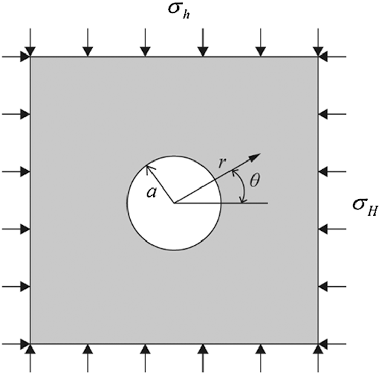
Figure 1: A cylindrical cavity of radius a under the action of biaxial stresses. Plane strain model. Stress
Although some works aiming at explaining the mechanisms of interaction among HF, NF, and cavity have been done by researchers, it still lacks a systematic study and deeper understanding of crucial factors that influence the hydraulic fracturing efficiency in fracture-cavity reservoirs. On the other hand, existing studies mainly focus on simple geometrical configuration, and the study of the influence of cavity on hydraulic fractures in a wellbore is not available in the literature. In this study, the XFEM proposed by Belytschko et al. [23] is adopted to describe the displacement field around fractures and cavities, the intersection between an HF and an NF, and the penetration of a fracture into a cavity. Consequently, the tedious remeshing process can be avoided after the propagation of fractures [10]. The fluid flow within fractures is described by Reynold’s equation [9] which is discretized using the FEM. Afterward, the displacements of all solid nodes including enriched nodes, and the pressure distribution of all fluid nodes along the hydro-fracture are obtained by solving the fully-coupled governing equations [10] using the Newton–Raphson (N–R) method.
This paper is presented as follows. The description of the numerical model is given in Section 2. Implementation and validation of the proposed numerical model are presented in Section 3. Mechanisms and factors that govern the propagation behavior of hydraulic fractures around natural cavities are systematically studied in Section 4. Major conclusions are summarized in Section 5.
2 Description of the Numerical Model
A shown in Fig. 2, we consider the domain
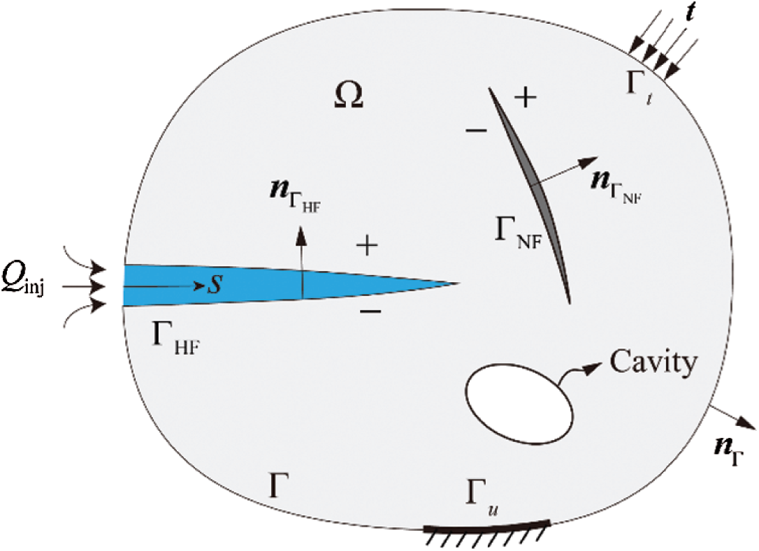
Figure 2: Illustration of the hydraulic fracturing problem in the fracture-cavity reservoir
According to the linear elastic assumption of rock formation, the governing equations for quasi-static deformation can be written as [10]
where
The fluid flow along the hydraulic fracture can be described by Reynold’s equation [25]
where w, t, p, and
where CL is the fluid leak-off coefficient, and
After introducing the trial function u(x, t) and test function
Besides, by introducing the test function
Spatial and time discretization of Eqs. (5) and (6) can be found in our previous work [10]. Afterward, the solid–fluid coupling problem is governed by Eqs. (2) and (3) can be iteratively solved by using the Newton-Raphson method [10].
2.2 Extended Finite Element Method
In this paper, we use the XFEM to describe the displacement field around fractures and cavities. By simply introducing additional degrees of freedoms (DOFs), i.e., the enriched DOFs, the remeshing and data mapping between old and new meshes can be avoided [27] and the demand on mesh refinement around fracture tip can be greatly alleviated owing to the fracture tip enrichment function, leading to a significant reduction of the problem complexity and computational time. This is a substantial improvement for numerical simulation of problems containing strong or weak discontinuities, especially for simulation cases where a large number of fractures and caves are involved. Since its introduction in 1999 [23,27], the XFEM has been adopted by many researchers to study various kinds of problems related to hydraulic fracturing. For problems where the intersection of an HF and an NF, as well as the intersection of a fracture and a cavity, are considered, the displacement of a point x inside the domain
in which NI denotes the shape function of node I, Sall denotes the set of all nodes whose displacement vector is denoted by
where (r,
which indicates that
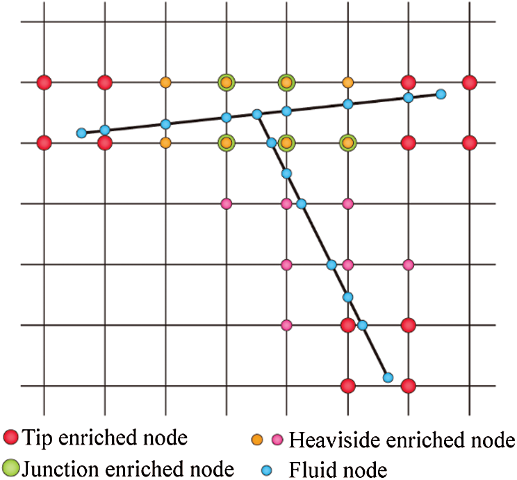
Figure 3: Depiction of the enriched nodes for a T-shaped junction formed by two fractures. The fluid nodes are also shown. Nodes whose support domain contains two intersected fractures should be selected as junction enriched nodes
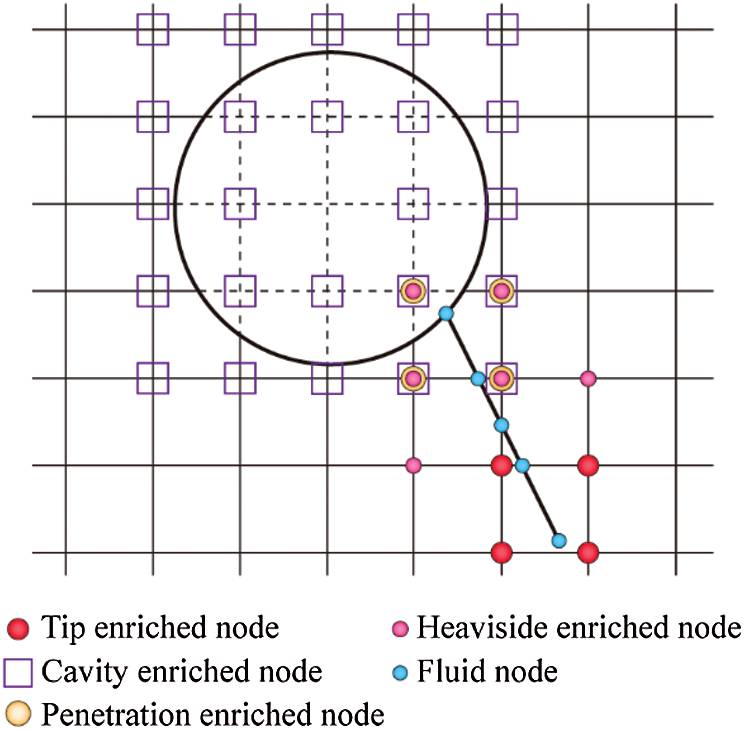
Figure 4: Depiction of the enriched nodes for penetration of a fracture into a cavity. The fluid nodes are also shown. Nodes whose support domain contains both the boundary of the cavity and the fracture should be selected as penetration enriched nodes
2.3 Frictional Behaviors of Natural Fractures
Frictional and cemented fractures are two common types of natural fractures in reservoirs [24]. In this article, the frictional natural fractures are considered due to their stronger influence on the creation of the fracture network in comparison with cemented natural fractures [24]. Thus, to avoid embedding of fracture surfaces under the effect of compressive stress, the frictional behaviors of natural fractures must be considered. The no-embedding conditions of fracture surfaces can be expressed as [28]
where
where
In this article, the penalty function method together with the Newton–Raphson method [10] is adopted to consider the frictional force and the contact status in the simulation. For each Newton–Raphson iteration Step i, the following linear system is solved
and the global conventional DOFs vector
until the following convergence criterion is satisfied
In Eq. (12),
In Eq. (15), N is the matrix of shape function, B is the matrix of shape function derivatives, D is the stress-strain matrix, and
where kN and kT are the penalty parameters in the normal and tangential directions, respectively, and
2.4 Fracture Propagation Criterion
The widely adopted maximum hoop-stress criterion [30] related to Mode-I (KI) and Mode-II (KII) stress intensity factors (SIFs) is used to check whether and along which direction the fracture will propagate
where
If Ke exceeds the fracture toughness of reservoirs (KIC), the fracture will propagate and deflect by the angle
3 Model Implementation and Validation
The proposed numerical model is implemented in an in-house Fortran code called PhiPsi (http://phipsi.top/): A general-purpose XFEM-based program. The level set method [33] is used to describe fractures and cavities, and to track the growth of fractures. The compressed sparse row (CSR) format is used to store global system matrices with optimized memory consumption. For the simulation cases where frictional natural fractures are considered (Section 4.1.6), two types of Newton–Raphson iteration loops are performed [10]. The outer loop solves the solid–fluid coupling equations (Eqs. (2) and (3)), and the inner loop determines the contact status of natural frictional fractures [10]. For each Newton–Raphson iteration step, an iterative solver called Lis [34] is adopted to solve the linear system. The flowchart of the simulation algorithm [10] is shown in Fig. 5.
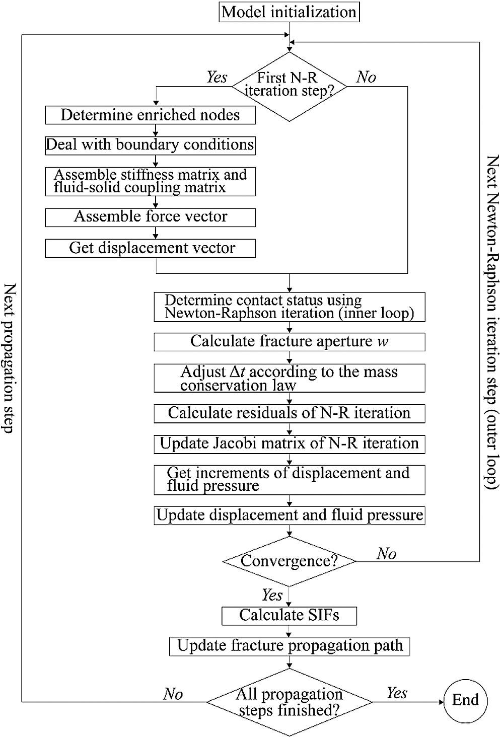
Figure 5: Flowchart of the simulation algorithm
The validation of the presented numerical model without considering cavities has been sufficiently conducted in our previous articles [9,10,24,35]. In this section, the propagation of an initial fracture towards a cavity in a panel under the action of tensile load is studied to verify the capacity of the proposed model for predicting interactions between fractures and cavities. As illustrated in Fig. 6, the bottom of a plane stress panel is fixed and the top of the panel is subjected to tensile stress
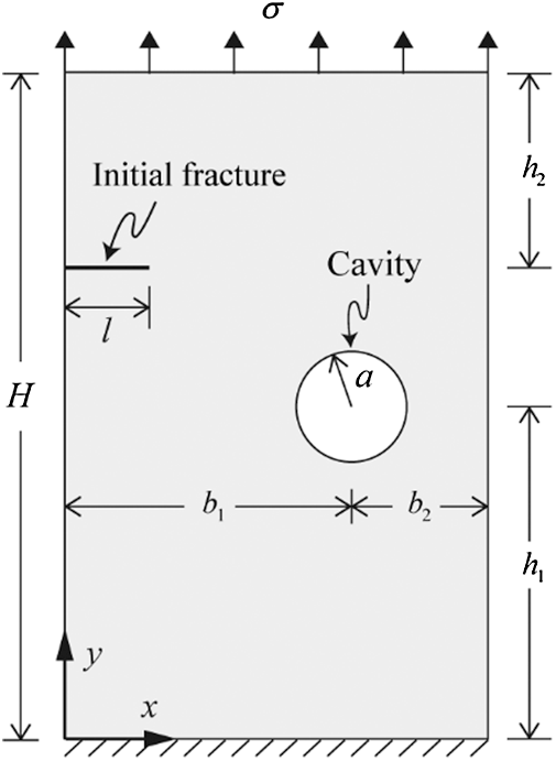
Figure 6: Illustration of a panel that contains a fracture of initial length l and a cavity of radius a. The bottom of the panel is fixed and the top of the panel is subjected to tensile stress
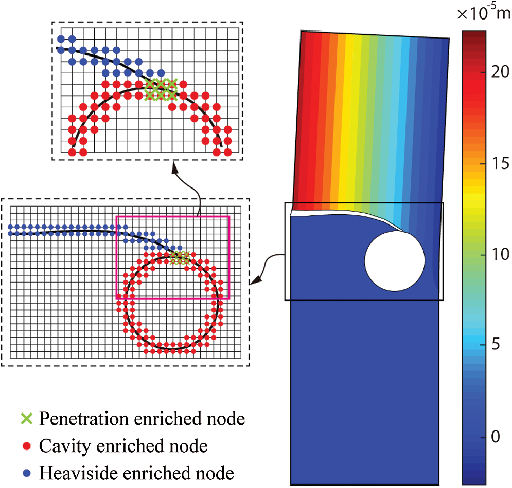
Figure 7: Vertical displacement field and enriched nodes of the last propagation step when the fracture penetrates into the cavity. The deformation scale factor is 200
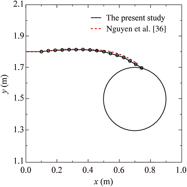
Figure 8: Comparison of the propagation path with the existing simulation result in the literature. The black dots represent locations of the fracture tip during the propagation process. The black circle represents the cavity
The simulation of a frictional natural fracture of length 10 m in a plane strain plate under the action of compressive stress will be performed to verify the frictional model presented in Section 2.3. As shown in Fig. 9a fracture at 50
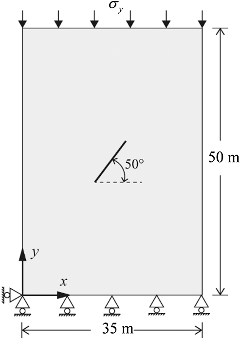
Figure 9: Illustration of a frictional natural fracture in a plane strain plate under the action of compressive stress
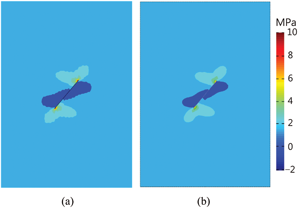
Figure 10: Contours of maximum principal stress obtained from: (a) The XFEM solution and (b) The FEM solution
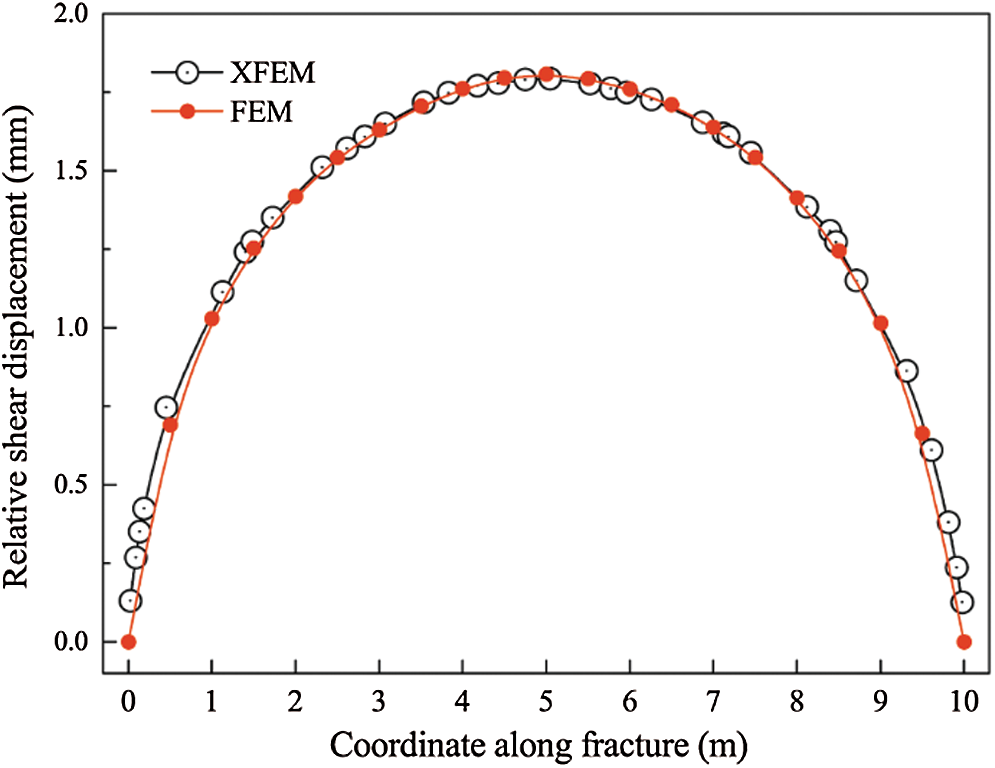
Figure 11: Comparison of relative shear displacement between fracture surfaces
4.1 Interactions between Hydraulic Fracture and Cavity
In this section, interactions between hydraulic fracture and cavity will be studied via a simple model shown in Fig. 12. The influence of factors including in-situ stress, viscosity of the injected fluid, pumping rate of the fluid, size of the cavity, shape of the cavity, and natural fracture will be thoroughly investigated. The size of the model is
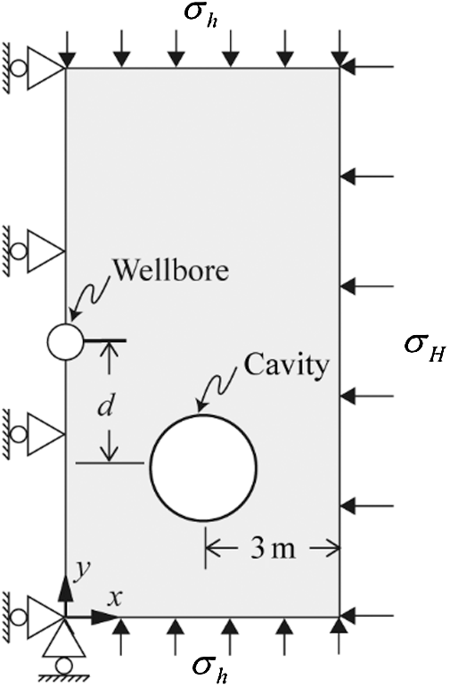
Figure 12: Geometry and boundary conditions of the model studied in Section 4.1. Plane strain condition is assumed
The strongly deflected fracture propagation path and the stress distribution in y-direction are shown in Fig. 13. It can be conjectured that if there is no cavity in this example, the hydraulic fracture will propagate horizontally, i.e., in the direction orthogonal to the minimum principal stress
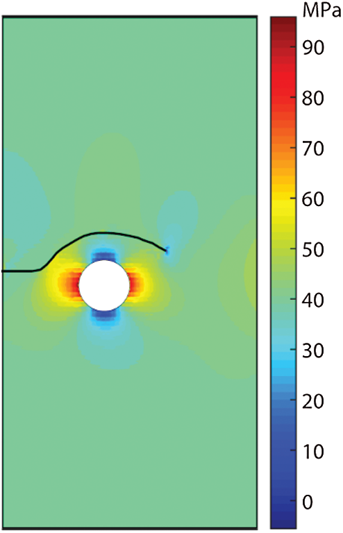
Figure 13: Propagation path of the hydraulic fracture and the stress distribution in y-direction. A positive value indicates compressive stress
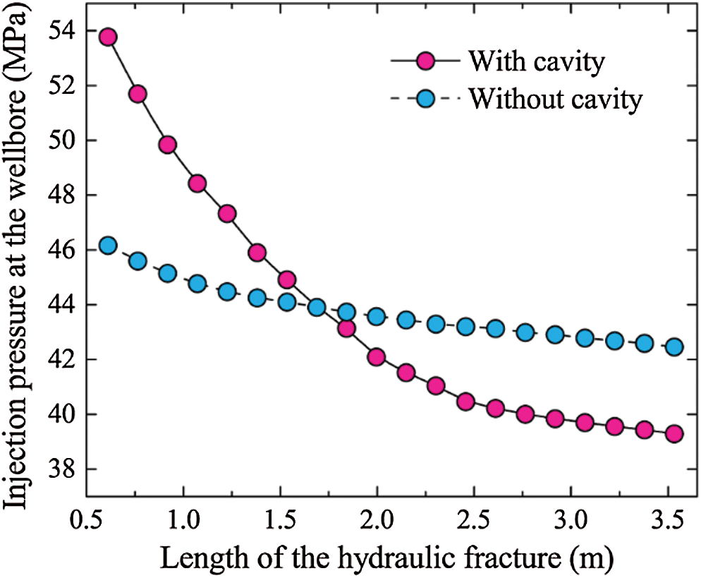
Figure 14: Comparison of the injection pressure at the wellbore between the scenarios with and without the cavity
4.1.1 Effects of In-situ Stress
The level of in-situ stress increases with the increase of the reservoir depth. On the other hand, as discussed in the introduction section, the stress field surrounding the cavity is strongly affected by the lateral stress coefficient
Table 1: Different cases of in-situ stress
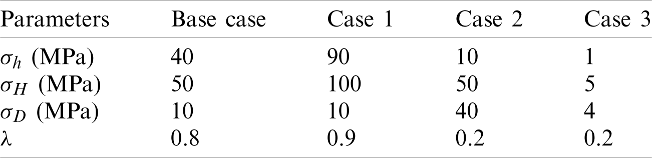
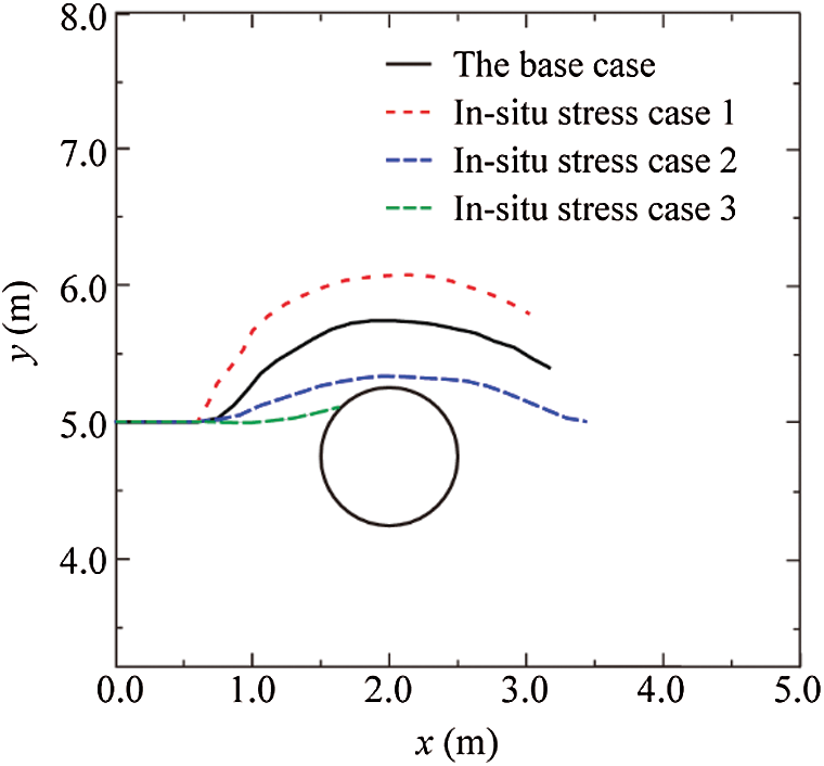
Figure 15: Comparison of fracture propagation paths for three different cases of in-situ stress
4.1.2 Effects of Fluid Viscosity
Fluid viscosity is an important factor in hydraulic fracturing treatments. In this section, a fluid of higher viscosity, 0.1
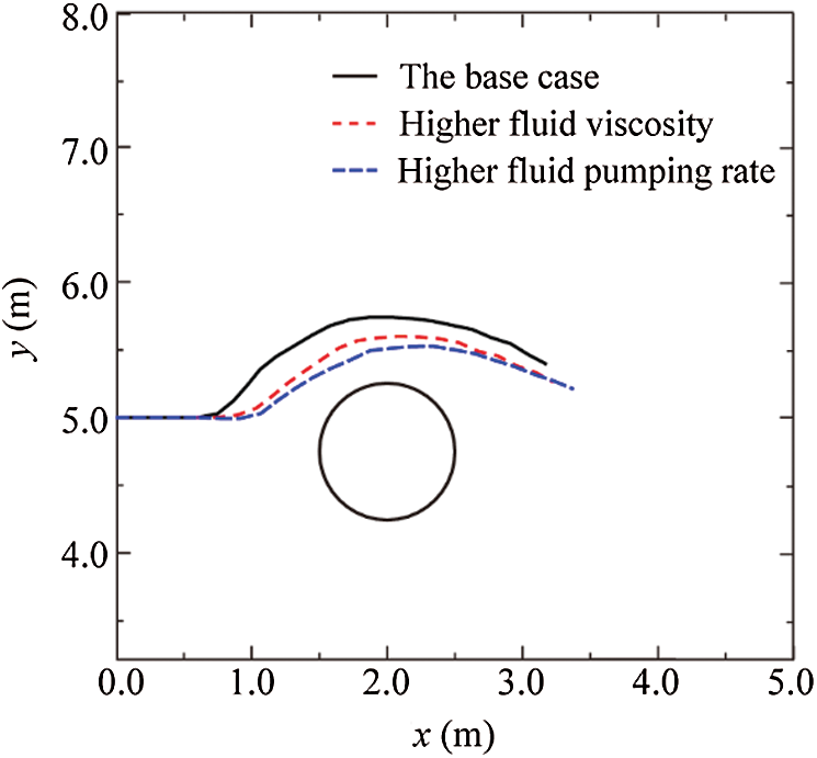
Figure 16: Comparison of fracture propagation paths for higher fluid viscosity and higher fluid pumping rate with the base case
4.1.3 Effects of Fluid Pumping Rate
In this section, we investigate the effect of another key factor, the fluid pumping rate. Different from the base simulation case, a higher pumping rate, 0.01 m2/s, is applied. The simulated propagation path is also shown in Fig. 16 in which a smoother path can be seen compared to the base case. Therefore, it can be concluded that a high fluid pumping rate is able to attenuate the effect of the cavity, and thus benefits the propagation of the hydraulic fracture along its original direction. This phenomenon can be explained with the aid of the analytical solution of the KGD model [38] which reveals that a higher pumping rate results in increased fluid pressure.
Cavities with greatly different scales are widely distributed in fracture-cavity carbonate reservoirs [2]. In this section, we consider a smaller cavity of radius 0.3 m to study the effect of cavity size. The simulated path is illustrated in Fig. 17. Just as expected, for a smaller cavity, its effect is significantly weakened in comparison with the base case. Besides, it is worth noting that the hydraulic fracture does not start to deflect until its tip comes into the zone near enough to the cavity.
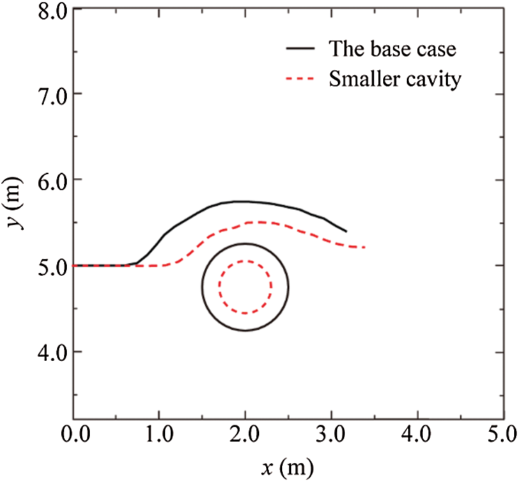
Figure 17: Comparison of fracture propagation paths for different sizes of cavities. The red dotted circle represents the smaller cavity
Natural cavities are of quite irregular shapes in fracture-cavity reservoirs [2]. In this section, two elliptical cavities oriented in different directions (a horizontal elliptical cavity and a vertical elliptical cavity) are studied to investigate the effect of cavity shape. The elliptical and circular cavities have the same area. The eccentricity of both ellipses takes a value of
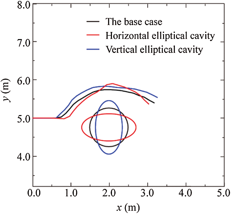
Figure 18: Comparison of fracture propagation paths for cavities of different shapes
4.1.6 Effects of Natural Fractures
As shown in Fig. 19, the influence of natural fractures will be investigated through four different cases. All of the natural fractures have the same length of 0.6 m and are positioned along the normal direction of the cavity. The friction angle of the fracture surface and the cohesive strength of the natural fracture are
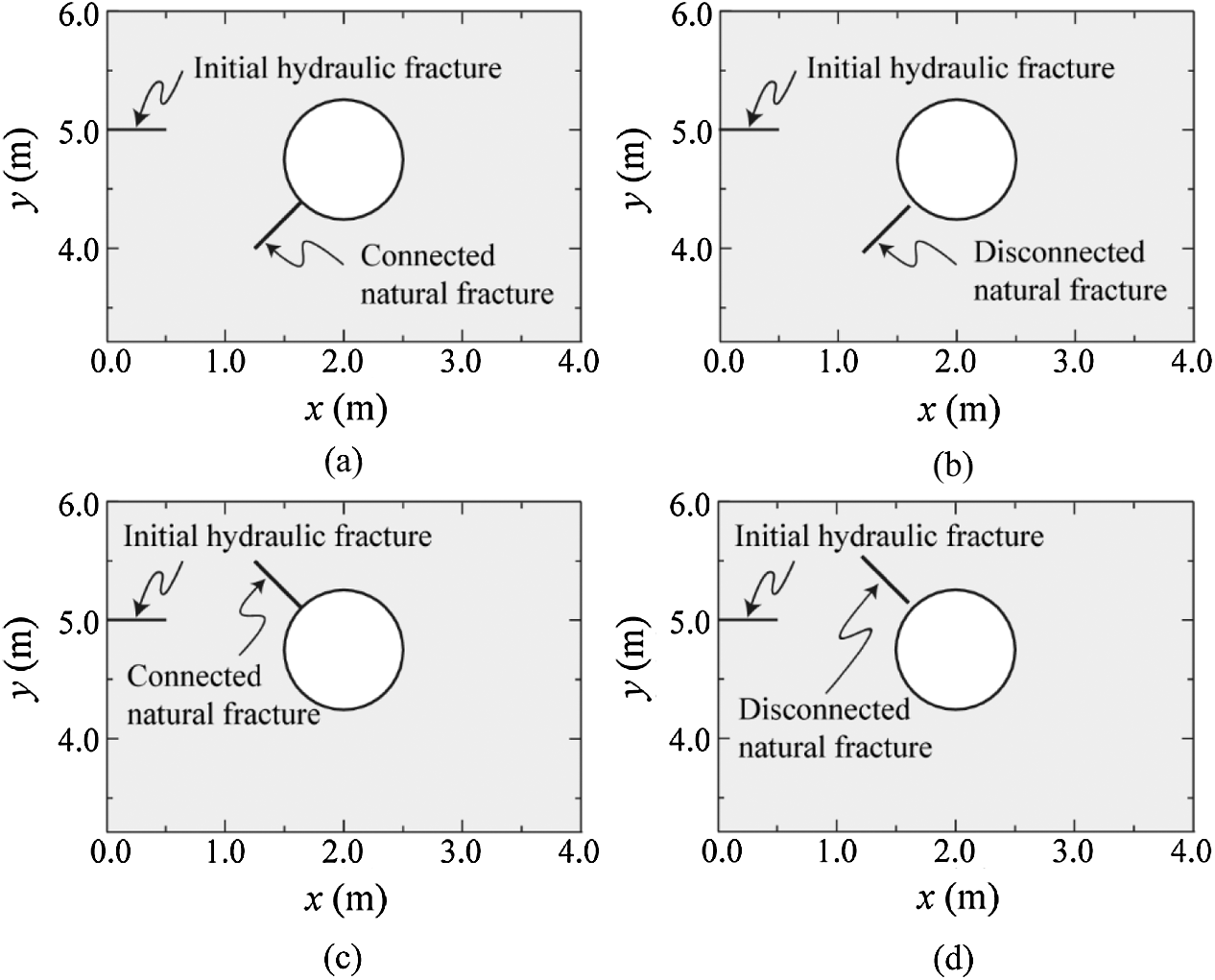
Figure 19: Illustration of different cases of natural fracture around the cavity: (a) The natural fracture with an angle of
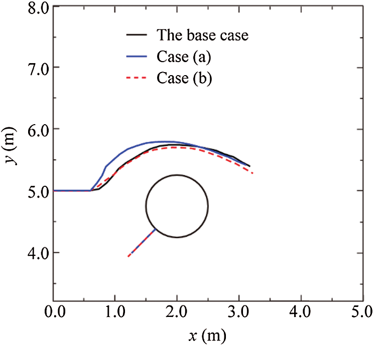
Figure 20: Comparison of fracture propagation paths for cavities with connected and disconnected natural fractures: Case (a) and Case (b)
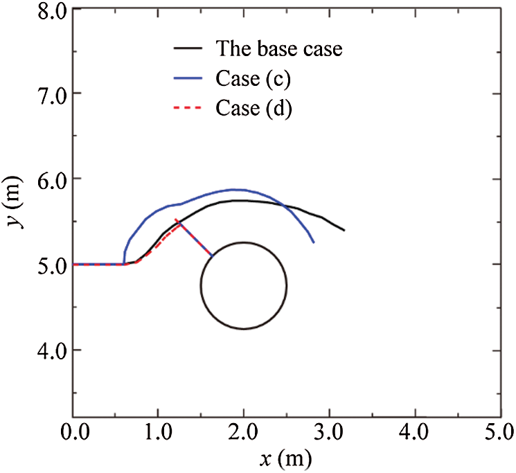
Figure 21: Comparison of fracture propagation paths for cavities with connected and disconnected natural fractures: Case (c) and Case (d). In Case (d), the hydraulic fracture is arrested by the natural fracture
4.2 Effects of Cavity on Hydraulic Fracturing in a Wellbore
This section is aimed to study the influence of cavity on hydraulic fracturing in a wellbore. As illustrated in Fig. 22, for the sake of simplicity, only the first two stages (Stages 1 and 2) are considered [9]. The size of the model is
The propagation paths of Stages 1 and 2 fractures for both cases without and with cavity are illustrated in Fig. 23. The stress contours in x-direction for cases without and with cavity are shown in Figs. 24a and 24b, respectively. These simulation results reveal that the existing cavity between two sequential fracturing stages significantly influences the propagation paths. For the case without the cavity, the Stage-2 hydraulic fracture curves away from the straight Stage-1 fracture because of the stress shadow effects [41] caused by the propped Stage-1 fracture, and the final paths are symmetrical about the wellbore. For the case with cavity, the Stage-1 fracture deviates leftward for both the upper and lower fracture tips, and the fracture path below the wellbore (y < 0) is more curved than that above the wellbore (y > 0). For the subsequent Stage-2 fracture, its fracture tip above the wellbore (y > 0) grows away from the previous Stage-1 fracture; However, the fracture tip below the wellbore (y < 0) firstly grows towards and then away from Stage-1 fracture. Besides the propagation paths, the stress fields are also quite distinct. The maximum stress values in x-direction for the cases without and with cavity are 36.1 and 43.2 MPa, respectively. For the case shown in Fig. 24b, both the maximum stress and the minimum stress in x-direction occur around the cavity. The maximum stress occurs on the upper and lower sides of the cavity, and the minimum stress occurs on the left and right sides of the cavity. The distinct propagation paths shown in Fig. 23 are a direct result of the stress concentration caused by the cavity.
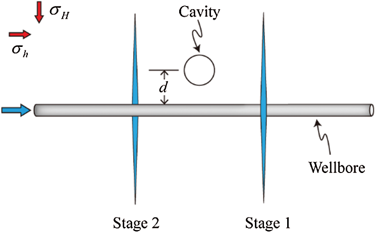
Figure 22: Illustration of two-stages sequential hydraulic fracturing in a wellbore. The cavity is placed between Stage-1 hydro-fracture and Stage-2 hydro-fracture with a vertical distance d to the wellbore
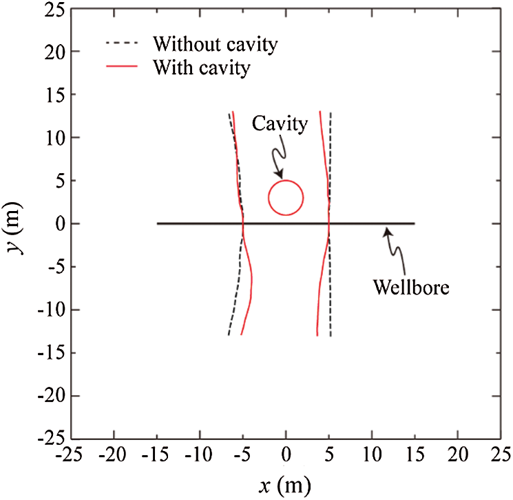
Figure 23: Propagation paths of Stage-1 fracture and subsequent Stage-2 fracture within a zone of size
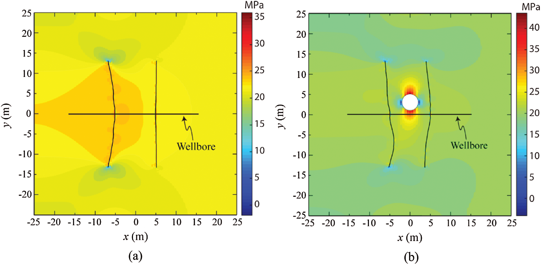
Figure 24: Stress contours in x-direction within a zone of size
In this paper, we established a fully-coupled numerical model to investigate the mechanisms of hydraulic fractures in fracture-cavity reservoirs using the XFEM. The Heaviside, cavity, fracture tip, T-shaped junction, and penetration enrichment functions are proposed to describe the displacement jump across the fracture surface, displacement discontinuity over the cavity boundary, singular displacement field near the fracture tip, intersection between the hydro-fracture and the natural fracture, and penetration of a fracture into the cavity, respectively. Hence, tedious remeshing can be avoided. The fluid flow within fractures is described by Reynold’s equation which is discretized using the FEM. Afterwards, the fully-coupled governing equations are solved iteratively using the Newton–Raphson method. After the validation of the proposed model in Section 3, several cases are simulated to investigate the effects of factors such as in-situ stress, fluid viscosity, fluid pumping rate, cavity size and shape, and natural fractures in Section 4.1. Besides, the effects of a cavity on the sequential hydraulic fracturing in a wellbore are studied in Section 4.2. According to the cases studied in this paper, the major conclusions can be reached as follows:
1. Both the lateral stress coefficient and the level of confining stress (or in-situ stress difference) have a strong influence on propagation paths of hydraulic fractures near cavities. A higher lateral stress coefficient can enhance the influence of the natural cavity, causing a more curved fracture path. However, lower confining stress or smaller in-situ stress difference can reduce this influence, and thus contributes to the penetration of the hydraulic fracture towards the cavity.
2. The fluid viscosity and fluid pumping rate are two dominant factors on the propagation path in hydraulic fracturing treatments when natural cavities are considered. Higher fluid viscosity and high fluid pumping rate are both able to attenuate the effect of the cavity, and thus benefit the propagation of the hydraulic fracture along its original direction.
3. The influence of a cavity depends not only on its size but also on its shape. Cavities of irregular shape (ellipse, for example) have a stronger influence on the propagation path of hydraulic fracture than regular circle cavity.
4. The frictional natural fracture disconnected from the cavity, even with a very small distance between the fracture tip and the cavity, has limited influence on the stress field around the cavity. Nevertheless, a frictional natural fracture connected to the cavity can significantly change the stress distribution around the cavity, thus dramatically deviates the hydraulic fracture from its original propagation direction.
5. Natural cavity existing between two adjacent fracturing stages will significantly influence the stress distribution between fractures and is more likely to result in irregular propagation paths compared to the case without cavity.
Availability of Data and Materials: The data that support the findings of this study are available from the corresponding author on reasonable request.
Funding Statement: This research was jointly funded by the National Natural Science Foundation of China (No. 51904111), the Natural Science Foundation of Jiangsu Province (No. BK20170457), the Open Fund for Jiangsu Key Laboratory of Advanced Manufacturing Technology (No. HGAMTL-1712), and the Natural Science Research of Institution of Higher Education of Jiangsu Province (No. 17KJA460003).
Conflicts of Interest: The authors declare that they have no conflicts of interest to report regarding the present study.
1. Khvatova, I. E., Renaud, A., Malyutina, G., Sansiev, G., Kuzilov, I. et al. (2012). Simulation of complex carbonate field: Double media vs. single media Kharyaga field case (Russian). SPE Russian Oil and Gas Exploration and Production Technical Conference and Exhibition, Society of Petroleum Engineers. Moscow, Russia. [Google Scholar]
2. Li, Y., Hou, J., Li, Y. (2016). Features and classified hierarchical modeling of carbonate fracture-cavity reservoirs. Petroleum Exploration and Development, 43(4), 655–662. DOI 10.1016/S1876-3804(16)30076-3. [Google Scholar] [CrossRef]
3. Schrefler, B. A., Secchi, S., Simoni, L. (2006). On adaptive refinement techniques in multi-field problems including cohesive fracture. Computer Methods in Applied Mechanics and Engineering, 195(4–6), 444–461. DOI 10.1016/j.cma.2004.10.014. [Google Scholar] [CrossRef]
4. Song, C., Chen, Y., Wang, J. (2019). Experiment and simulation for controlling propagation direction of hydrofracture by multi-boreholes hydraulic fracturing. Computer Modeling in Engineering & Sciences, 120(3), 779–797. DOI 10.32604/cmes.2019.07000. [Google Scholar] [CrossRef]
5. Tang, H., Wang, S., Zhang, R., Li, S., Zhang, L. et al. (2019). Analysis of stress interference among multiple hydraulic fractures using a fully three-dimensional displacement discontinuity method. Journal of Petroleum Science and Engineering, 179(3), 378–393. DOI 10.1016/j.petrol.2019.04.050. [Google Scholar] [CrossRef]
6. Liu, Z., Lu, Q., Sun, Y., Tang, X., Shao, Z. et al. (2019). Investigation of the influence of natural cavities on hydraulic fracturing using phase field method. Arabian Journal for Science and Engineering, 44(12), 10481–10501. DOI 10.1007/s13369-019-04122-z. [Google Scholar] [CrossRef]
7. Zhou, S., Zhuang, X., Rabczuk, T. (2019). Phase-field modeling of fluid-driven dynamic cracking in porous media. Computer Methods in Applied Mechanics and Engineering, 350(6), 169–198. DOI 10.1016/j.cma.2019.03.001. [Google Scholar] [CrossRef]
8. Shimizu, H., Murata, S., Ishida, T. (2011). The distinct element analysis for hydraulic fracturing in hard rock considering fluid viscosity and particle size distribution. International Journal of Rock Mechanics and Mining Sciences, 48(5), 712–727. DOI 10.1016/j.ijrmms.2011.04.013. [Google Scholar] [CrossRef]
9. Shi, F., Wang, X., Liu, C., Liu, H., Wu, H. (2016). A coupled extended finite element approach for modeling hydraulic fracturing in consideration of proppant. Journal of Natural Gas Science and Engineering, 33(5), 885–897. DOI 10.1016/j.jngse.2016.06.031. [Google Scholar] [CrossRef]
10. Shi, F., Wang, X., Liu, C., Liu, H., Wu, H. (2017). An XFEM-based method with reduction technique for modeling hydraulic fracture propagation in formations containing frictional natural fractures. Engineering Fracture Mechanics, 173, 64–90. DOI 10.1016/j.engfracmech.2017.01.025. [Google Scholar] [CrossRef]
11. Cheng, L., Luo, Z., Yu, Y., Zhao, L., Zhou, C. (2019). Study on the interaction mechanism between hydraulic fracture and natural karst cave with the extended finite element method. Engineering Fracture Mechanics, 222(9), 106680. DOI 10.1016/j.engfracmech.2019.106680. [Google Scholar] [CrossRef]
12. He, B. (2019). Hydromechanical model for hydraulic fractures using XFEM. Frontiers of Structural and Civil Engineering, 13(1), 240–249. DOI 10.1007/s11709-018-0490-6. [Google Scholar] [CrossRef]
13. Wang, D., Zlotnik, S., Diez, P., Ge, H., Zhou, F. et al. (2020). A numerical study on hydraulic fracturing problems via the proper generalized decomposition method. Computer Modeling in Engineering & Sciences, 122(2), 703–720. DOI 10.32604/cmes.2020.08033. [Google Scholar] [CrossRef]
14. Kolawole, O., Ispas, I. (2020). Interaction between hydraulic fractures and natural fractures: Current status and prospective directions. Journal of Petroleum Exploration and Production Technology, 10(4), 1613–1634. DOI 10.1007/s13202-019-00778-3. [Google Scholar] [CrossRef]
15. Taleghani, A. D., Gonzalez, M., Shojaei, A. (2016). Overview of numerical models for interactions between hydraulic fractures and natural fractures: Challenges and limitations. Computers and Geotechnics, 71(3), 361–368. DOI 10.1016/j.compgeo.2015.09.009. [Google Scholar] [CrossRef]
16. Yu, H. S. (2020). Cavity expansion methods in geomechanics. Springer, Dordrecht: Kluwer. [Google Scholar]
17. Luo, Z., Zhang, N., Zhao, L., Zeng, J., Liu, P. et al. (2020). Interaction of a hydraulic fracture with a hole in poroelasticity medium based on extended finite element method. Engineering Analysis with Boundary Elements, 115(4), 108–119. DOI 10.1016/j.enganabound.2020.03.011. [Google Scholar] [CrossRef]
18. He, B., Zhuang, X. (2018). Modeling hydraulic cracks and inclusion interaction using XFEM. Underground Space, 3(3), 218–228. DOI 10.1016/j.undsp.2018.04.005. [Google Scholar] [CrossRef]
19. Wang, H., Tang, X., Luo, Z., Liu, P. (2018). Investigation of the fracture propagation in fractured-vuggy reservoirs. 52nd U.S. Rock Mechanics/Geomechanics Symposium, American Rock Mechanics Association. Seattle, Washington, USA. [Google Scholar]
20. Zhao, H., Xie, Y., Zhao, L., Liu, Z., Li, Y. et al. (2020). Simulation of mechanism of hydraulic fracture propagation in fracture-cavity reservoirs. Chemistry and Technology of Fuels and Oils, 55(6), 814–827. DOI 10.1007/s10553-020-01096-9. [Google Scholar] [CrossRef]
21. Al-Nakhli, A. R. (2015). Chemically-Induced pressure pulse: A new fracturing technology for unconventional reservoirs. SPE Middle East Oil & Gas Show and Conference, Society of Petroleum Engineers. Manama, Bahrain. [Google Scholar]
22. Wang, Y., Li, X., Zhao, B., Zhang, Z. (2020). 3D numerical simulation of pulsed fracture in complex fracture-cavitied reservoir. Computers and Geotechnics, 125(6), 103665. DOI http://dx.doi.org/10.1016/j.compgeo.2020.103665. [Google Scholar]
23. Belytschko, T., Black, T. (1999). Elastic crack growth in finite elements with minimal remeshing. International Journal for Numerical Methods in Engineering, 45, 601–620. DOI http://dx.doi.org/10.1002/(SICI)1097-0207(19990620)45:5. [Google Scholar]
24. Wang, X., Shi, F., Liu, C., Lu, D., Liu, H. et al. (2018). Extended finite element simulation of fracture network propagation in formation containing frictional and cemented natural fractures. Journal of Natural Gas Science and Engineering, 50(5), 309–324. DOI 10.1016/j.jngse.2017.12.013. [Google Scholar] [CrossRef]
25. Adachi, J., Siebrits, E., Peirce, A., Desroches, J. (2007). Computer simulation of hydraulic fractures. International Journal of Rock Mechanics and Mining Sciences, 44(5), 739–757. DOI 10.1016/j.ijrmms.2006.11.006. [Google Scholar] [CrossRef]
26. Carter, R. D. (1957). Derivation of the general equation for estimating the extent of the fractured area. Drilling and Production Practices, pp. 261–270. Dallas: American Petroleum Institute. [Google Scholar]
27. Moës, N., Dolbow, J., Belytschko, T. (1999). A finite element method for crack growth without remeshing. International Journal for Numerical Methods in Engineering, 46(1), 131–150. DOI 10.1002/(SICI)1097-0207(19990910)46:1. [Google Scholar] [CrossRef]
28. Wrigger, P. (2006). Computational contact mechanics. Second edition. Berlin, Heidelberg: Springer. [Google Scholar]
29. Khoei, A. R., Nikbakht, M. (2007). An enriched finite element algorithm for numerical computation of contact friction problems. International Journal of Mechanical Sciences, 49(2), 183–199. DOI 10.1016/j.ijmecsci.2006.08.014. [Google Scholar] [CrossRef]
30. Erdogan, F., Sih, G. C. (1963). On the crack extension in plates under plane loading and transverse shear. Journal of Biomechanical Engineering-Transactions, ASME, 85(4), 519–525. DOI 10.1115/1.3656897. [Google Scholar] [CrossRef]
31. Moran, B., Shih, C. F. (1987). Crack tip and associated domain integrals from momentum and energy balance. Engineering Fracture Mechanics, 27(6), 615–642. DOI 10.1016/0013-7944(87)90155-X. [Google Scholar] [CrossRef]
32. Gu, H., Weng, X., Lund, J. B., Mack, M. G., Ganguly, U. et al. (2012). Hydraulic fracture crossing natural fracture at nonorthogonal angles: A criterion and its validation. SPE Production & Operation, 27(1), 20–26. DOI 10.2118/139984-PA. [Google Scholar] [CrossRef]
33. Chessa, J., Belytschko, T. (2004). Arbitrary discontinuities in space-time finite elements by level sets and X-FEM. International Journal for Numerical Methods in Engineering, 61(15), 2595–2614. DOI 10.1002/nme.1155. [Google Scholar] [CrossRef]
34. Nishida, A. (2010). Experience in developing an open source scalable software infrastructure in Japan. Computational Science and Its Applications, vol. 6017, pp. 448–462. Berlin, Heidelberg: Springer. [Google Scholar]
35. Shi, F., Wang, X., Liu, C., Liu, H., Wu, H. (2018). An XFEM-based numerical model to calculate conductivity of propped fracture considering proppant transport, embedment and crushing. Journal of Petroleum Science and Engineering, 167(5), 615–626. DOI 10.1016/j.petrol.2018.04.042. [Google Scholar] [CrossRef]
36. Nguyen, N. T., Bui, T. Q., Zhang, C., Truong, T. T. (2014). Crack growth modeling in elastic solids by the extended meshfree Galerkin radial point interpolation method. Engineering Analysis with Boundary Elements, 44, 87–97. DOI 10.1016/j.enganabound.2014.04.021. [Google Scholar] [CrossRef]
37. Peng, S., Zhang, Z., Mou, J., Zhao, B., Liu, Z. et al. (2018). Hydraulic fracture simulation with hydro-mechanical coupled discretized virtual internal bond. Journal of Petroleum Science and Engineering, 169(3), 504–517. DOI 10.1016/j.petrol.2018.05.070. [Google Scholar] [CrossRef]
38. Hu, J., Garagash, D. I. (2010). Plane-strain propagation of a fluid-driven crack in a permeable rock with fracture toughness. Journal of Engineering Mechanics, 136(9), 1152–1166. DOI 10.1061/(ASCE)EM.1943-7889.0000169. [Google Scholar] [CrossRef]
39. Jeon, J., Bashir, M. O., Liu, J., Wu, X. (2016). Fracturing carbonate reservoirs: Acidising fracturing or fracturing with proppants? SPE Asia Pacific Hydraulic Fracturing Conference, Society of Petroleum Engineers. Beijing, China. [Google Scholar]
40. Rivers, M., Zhu, D., Hill, A. D. (2012). Proppant fracture conductivity with high proppant loading and high closure stress. SPE Hydraulic Fracturing Technology Conference, Society of Petroleum Engineers. The Woodlands, Texas, USA. [Google Scholar]
41. Roussel, N. P., Sharma, M. M. (2011). Strategies to minimize frac spacing and stimulate natural fractures in horizontal completions. SPE Annual Technical Conference and Exhibition, Denver, Colorado, USA. [Google Scholar]
 | This work is licensed under a Creative Commons Attribution 4.0 International License, which permits unrestricted use, distribution, and reproduction in any medium, provided the original work is properly cited. |