| Computer Modeling in Engineering & Sciences |
DOI: 10.32604/cmes.2021.014489
ARTICLE
Alcoholism Detection by Wavelet Energy Entropy and Linear Regression Classifier
1School of Electronic Science and Engineering, Nanjing University, Nanjing, 210093, China
2Department of Electrical Engineering, College of Engineering, Zhejiang Normal University, Jinhua, 321004, China
3Educational Information Center, Liming Vocational University, Quanzhou, 362000, China
*Corresponding Author: Yan Yan. Email: yanyan899@outlook.com
Received: 01 October 2020; Accepted: 08 January 2021
Abstract: Alcoholism is an unhealthy lifestyle associated with alcohol dependence. Not only does drinking for a long time leads to poor mental health and loss of self-control, but alcohol seeps into the bloodstream and shortens the lifespan of the body’s internal organs. Alcoholics often think of alcohol as an everyday drink and see it as a way to reduce stress in their lives because they cannot see the damage in their bodies and they believe it does not affect their physical health. As their drinking increases, they become dependent on alcohol and it affects their daily lives. Therefore, it is important to recognize the dangers of alcohol abuse and to stop drinking as soon as possible. To assist physicians in the diagnosis of patients with alcoholism, we provide a novel alcohol detection system by extracting image features of wavelet energy entropy from magnetic resonance imaging (MRI) combined with a linear regression classifier. Compared with the latest method, the 10-fold cross-validation experiment showed excellent results, including sensitivity
Keywords: Alcohol detection; wavelet energy entropy; linear regression classifier; cross-validation; computer-aided diagnosis
Alcoholism is one of the mental health problems. It is composed of two types: Alcohol dependence and alcohol abuse. Alcoholism could cause severe mental illness. Females are generally more vulnerable than males to the harmful effects of alcohol, because of their lower ability to metabolize alcohol, smaller body mass, and a higher proportion of body adipose tissue [1–3]. Many people are currently suffering from alcohol abuse. Many people believe that alcohol can relieve fatigue and relieve stress, or they can escape from reality. They often ignore the huge invisible damage it can do to their internal organs. Not only are overexcitability and aggressive mental disorders manifest themselves, but neurological damage and kidney failure are also major problems in alcoholism. Timely and accurate alcoholism tests can avoid prolonged heavy alcohol dependence and reduce the risk of acute kidney injury. For young people in their prime, alcohol abuse is a serious factor affecting their physical development throughout their lives. Heavy drinking can affect brain development, leading to memory loss and concentration problems. At the same time, the immature development of young people leads to the poor ability of each organ to deal with alcohol, which may easily lead to the hidden danger of fatty liver or cirrhosis. Alcohol is often essential for many young people’s celebrations or activities. They are encouraged to drink to avoid being excluded and discriminated against by their peers. In such a bad drinking environment, more young people are likely to be psychologically hard to get rid of the desire for compulsory drinking, thus falling into the harm of alcohol poisoning.
According to the World Health Organization, about three million people die each year from excessive drinking. Alcohol accounts for 5.1% of the global burden of disease. In the 2016 statistics, the global per capita alcohol consumption of aged 15 or older is around 6.4 litres, while Europe, the Americas and the Western Pacific region are far above the world’s average alcohol consumption levels, around 9.8 litres, 8.0 litres and 7.3 litres. Deaths due to excessive alcohol consumption account for 10% of all deaths in the same age group, and mortality and hospitalization rates are also higher among the poor, suggesting that vulnerable groups are more likely to be alcohol-dependent. It is regrettable that among the 155 countries that responded to the survey, there is a significant lack of postgraduate training courses to treat drug abuse, and that only about 15 percent of the countries have preventive measures.
The main causes of alcohol abuse are dull daily habits and stress. Avoiding excessive alcohol exposure in the early stages of alcoholism is the best way to protect people from the effects of alcoholism. Therefore, it is necessary to replace the daily drinking entertainment with healthier activities. Finding hobbies appropriately, replacing alcohol as a boring pastime with something meaningful, and reducing unnecessary drinking in daily life are all helpful to improve drinking habits. Controlling alcohol consumption in the early stage can effectively curb alcohol dependence, and the symptoms of alcohol abuse in the early stage are easy to miss the best time for self-adjustment once they are ignored.
Alcoholism influences all parts of the body, and it affects the brain. The size of gray matter (GM) and white matter (WM) of alcoholism patients are reportedly less than age-matched controls [4], and this shrinkage can be observed using magnetic resonance imaging (MRI). Thus, this paper aims to develop an artificial intelligence (AI) and MRI based alcoholism detection system (ADS).
Recently, many ADSs were reported. Hou [5] used Hu moment invariant (HMI) as feature extractor, and used an improved particle swarm optimization (IPSO) as classifier. The detection system developed is more accurate than genetic algorithm, firefly algorithm and particle swarm optimization algorithm. Yang [6] also used Hu moment invariant to input the seven feature results into two classifiers, the twin support vector machine and the generalized eigenvalue proximal support vector machine. He employed several different machine learning techniques, and found support vector machine (SVM) gives the best result. Jiang [7] used pseudo Zernike moment (PZM) as the image feature combined with kernel support vector machine for intelligent pathological brain detection. Chen et al. [8] used weighted fractional Fourier transform (WFFT) to extract the magnetic resonance image spectrum information, and then reduced the spectral characteristics through principal component analysis. The results of
The contribution of this study is to put forward a new alcohol detection method based on computer vision and image processing [15–19] to reduce the difficulty for physicians to diagnose patients with alcoholism. We propose a new wavelet energy entropy method based on which the energy information in the signal or system can be represented as image features. In addition, we combine a simple algorithm with a high-speed linear regression classifier. The performance was tested by calculating the mean value and standard deviation through the use of 10-fold cross-validation. Finally, an experiment is given to explain how to choose the optimal decomposition level of the hyper-parameter, namely the wavelet energy entropy.
Our method first obtains the image features of the magnetic resonance imaging (MRI) data in a higher-dimensional space through wavelet energy entropy, then the hyperplane of linear classification is used to separate the positive and negative samples, and establishes the model of the relationship between variables by linear regression. Finally, the 10-fold cross-validation is used to calculate the mean and standard deviation to verify the performance of the constructed model. Figs. 1a, 1b show two samples of the healthy brain and an alcoholic brain.
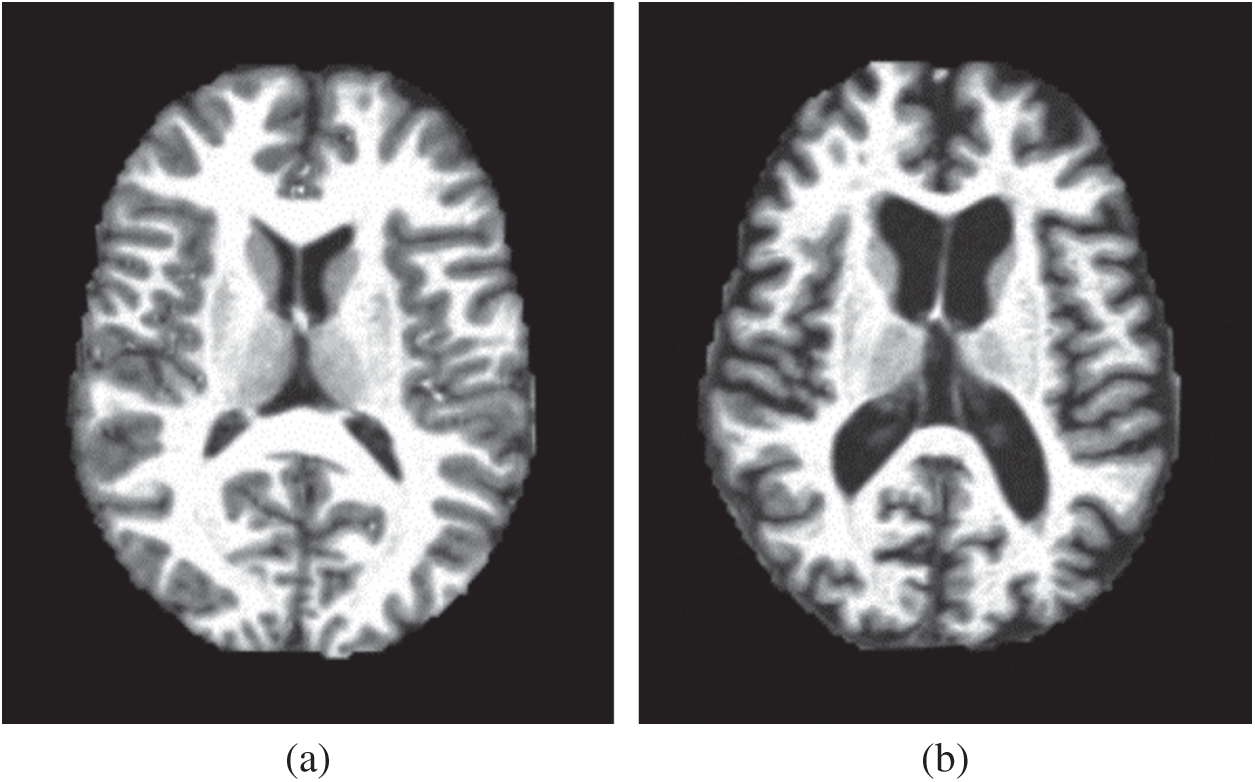
Figure 1: Two samples of our dataset (a) Healthy brain (b) Alcoholism brain
We use a new image feature extraction method [20,21]. Firstly, we collected the vibration signals of magnetic resonance imaging (MRI) of alcoholism and performed discrete wavelet transform. Then, we calculated the maximum energy through the wave coefficient and combined it with Shannon entropy to obtain the efficient classification feature—wavelet energy entropy (WEE). The traditional Fourier transform produces smooth results for non-stationary signals in both the time domain and frequency domain. The resulting value of the arbitrary component of the spectrum depends on the time domain waveform in
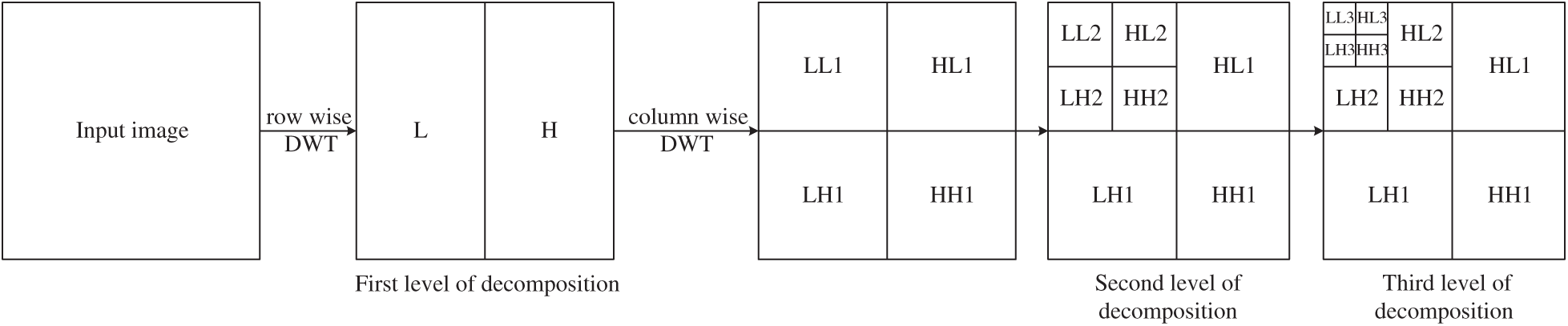
Figure 2: The process of discrete wavelet decomposition
Discrete wavelet transform has an excellent detection effect, which can achieve fast computation. Furthermore, it has the advantages of automatically adjustable time-frequency resolution for time-frequency domain analysis. The dimensionality of the discrete Wavelet transform coefficient [27,28] can be reduced by getting the wavelet energy feature by calculating the wavelet coefficients of the input image decomposition. The advantage of Shannon entropy is that it not only quantitatively measures the size of information, but also provides the theoretical optimal value for information coding [29–32]. Combined with the above optimal methods as the MRI image feature extraction, the reduced and accurate detection space can obtain high-quality feature vectors as the input signal of the classifier, improving the overall efficiency of the algorithm.
In the process of image extraction, we assume that the decomposition level of the wavelet coefficient of signal S(l, t) is l and the translation is t. The energy signal is represented by E(l, t), and we have:
Then the Shannon entropy of the energy coefficient E(l, t) is defined as WEE at l level,
2.2 Linear Regression Classifier
The Linear regression classifier (LRC) [33,34] is born from the concept that there is a linear relationship between features and classification results, which means that the sample of a particular object is classified by linear subspace. The nonlinear classification has the advantage of surface or combination of multiple hyperplanes owing to the lack of limitation, but its programming complexity increases greatly. In contrast, the LRC is simpler and has the ability of automatic learning, which makes the programming of its classifier easier and the operation efficiency is higher than that of the nonlinear classification method. The establish of a model based on LRC is widely used in data analysis as a supervised machine learning algorithm. There are many typical LRCs, including linear discriminant analysis, support vector machine [35–37], Logistic regression and so on.
The principle of LRC is to divide samples into positive and negative by a hyperplane that does not care about the dimension of space, and the most classical basic expression is y = wx. The model is a linear function of parameters, where x represents samples and w represents the weighted value. The LRC is mainly composed of two parts: One is the scoring function; the other is the loss function. The Score function is a mapping function from the original image to the category score, and the loss function is used to quantify the consistency between the predicted score of the classification tag and the real tag.
The category decision of this model is completed by summing up the product of the characteristics of each dimension and their respective weights. The simplest dichotomy we use is to make the data feature belong to [0, 1]. Therefore, a function is required to attribute the original data eigenvalues to a value set and map them to [0, 1].
We assume that the extracted image eigenvalues are located in the linear subspace in a specific category and that a data set Dj with a classified number of n is grouped into a set
It is not necessary to know the statistical information about the estimator and the measurement. The least square estimation method is used for parameter estimation because of its simplicity. Through least square estimation, the reconstruction coefficient rj is as follows:
Then we reconstructed image Aj of the alcoholism image,
The similarity of alcoholism images to the j-th class was estimated by the reconstruction error ej of the j-th class,
It is possible to assume an unknown picture of alcoholism I. By using all n-class models to calculate the reconstruction error, I is classified under the following label,
The LRC can intuitively express the relationship between independent variables and dependent variables according to the coefficients and give the interpretation of each variables. At the same time, LRC has the obvious advantages of fast modeling speed and running speed in case of large data volume. However, it is unavoidable that the LRC cannot fit the nonlinear data well. Therefore, it is necessary to first determine whether the variables are in linear relationship, to avoid the use of overly complex nonlinear classifiers on the one hand, and improve the efficiency of modeling on the other hand.
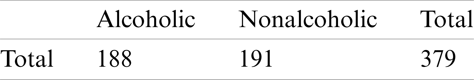
379 slices were obtained in which there are 188 alcoholic brain images and 191 non-alcoholic brain images. The division is shown in Tab. 1. The 10-fold cross-validation approach [38–40] is used here to evaluate the model.
Table 1: Dataset division into training, validation, and test sets
Compared with cross-validation [41,42] using the same number of folds in the total number of samples, 10-fold cross-validation greatly reduces the training complexity, because the former is only suitable for a small number of samples [43–46]. Therefore, 10-fold cross-validation is the most popular way to test the performance of a model.
The method first divides the data set into 10 folding subsets of the same size randomly as shown in Fig. 3. Nine of them are used as training sets to train the model, and the other part is used as test sets to evaluate the model. In such 10 iterations, each subset is rotated once as a test set, and the remaining subsets are used as training sets to obtain fair test results. The model obtained after training on each training set was tested on the corresponding test set. Each evaluation index’s results of the model were calculated and saved for 10 times, and the estimation of algorithm accuracy was obtained through average calculation [47–49].
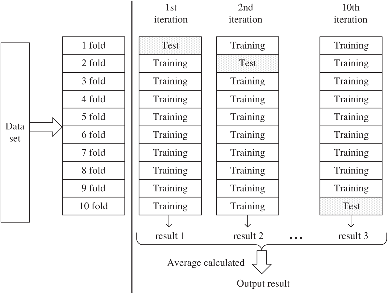
Figure 3: The process of 10-fold cross-validation
The single cross-validation results are less reliable because of possible variation. In contrast, the characteristic of regular repetition of 10-fold cross-validation makes the method reliable in verifying model performance. Although in some cases it is not substantially different from 5-fold or 20-fold cross-validation. However, there are still researches and theoretical evidence to prove that 10-fold cross-validation is an appropriate choice to prevent neural network from overfitting to obtain the best error estimate.
The process we realized was divided into three parts. First, the wavelet transform coefficient of the image was extracted, then the wavelet energy was calculated and the entropy value was obtained by combining Shannon entropy, and finally the feature vector obtained was classified as the input of the linear regression classifier. The statistical results of this model are obtained by using
During the experiment, we compared six indicators: Sensitivity (sen), specificity (spc), precision (pre), accuracy (acc), F1 score (F1) and Matthews correlation coefficient (MCC). To evaluate the classifier, the output of the classifier is compared with the ideal reference classification. Suppose the question was whether someone had alcohol poisoning. Some of them suffered from alcoholism, and the results of the classification tests correctly indicated that they were positive. We use RU for those who were included in the experiment with true positivity. People who have alcohol poisoning are not classified as patients on the test and the error we use FU for that is called false negative. Some people do not have the disease and the tests show they are truly negative, we call them RH. Finally, there may be healthy people who test positive-false-positive, which we will call FH.
Sensitivity represents the ratio of the correct markers in our program to all actual patients with alcoholism, and the formula is expressed as follows:
The accuracy value can usually clearly show the performance of our model. The formula for accuracy during the experiment is as follows:
However, the accuracy of the model is likely to be affected by the imbalance of positive and negative samples. Therefore, the single accuracy value cannot well reflect the overall situation of the model.
Specificity was the correct marker in the experiment for all real people who did not have the disease, and its expression formula is:
Precision is also one of the evaluation indexes for the predicted results. It mainly represents the percentage of the results predicted by the model as positive samples that are actually positive samples. The formula for the precision is as follows:
The high accuracy rate means that it can well reflect the stronger ability of the model to distinguish negative samples.
F1-score is the harmonic mean of accuracy and recall rates.
It mainly aims at the shortcomings of missing data caused by high accuracy rate caused by high threshold and the reduction of prediction accuracy caused by high recall rate.
MCC is a relatively balanced indicator that describes the correlation coefficient between the predicted results and the actual results. The expression formula of MCC is as follows:
One of its advantages is that it can also be used in the case of sample imbalance. It considers True Positives, False Positives, False Negatives and True Negatives as well. The value range of MCC is [ −1, 1]. A value of 1 means that the prediction is completely consistent with the actual result; a value of 0 means that the predicted result is lower than the random prediction result; and a value of −1 means that the predicted result is completely inconsistent with the actual result.
Wavelet transform is a local transform in time and frequency domain. It can extract information from signals effectively by means of multi-scale refinement analysis of functions or signals by means of scaling and shifting. Fourier transform is a tool of mutual transformation from time domain to frequency domain, and it is one of the most widely used and effective analytical methods in signal processing. After the appearance of wavelet analysis, it inherits and develops the features of Fourier transform localization, which is suitable for signal time-frequency analysis and processing, solves the defect of Fourier transform, and becomes a popular method in many application fields.
The Fourier transform is a global transformation, and the values of each point in the function affect the result of the transformation. In contrast to the Fourier transform, wavelets use local bases, and the coefficients are affected only by the points on the support of a particular base. This results in wavelets containing not only frequency information but also time information. The Fourier transform gives information in the one-dimensional frequency domain, which is a mixture of important features of frequency. However, the time information cannot be read directly from the frequency domain. The result of the wavelet transform is two-dimensional information, the horizontal axis is the time axis, and the vertical axis is the frequency. Therefore, a wavelet is very useful for analyzing instantaneous time-varying signals, and some features of the image can be fully highlighted through transformation.
The wavelet decomposition of magnetic resonance imaging is shown in the Fig. 4, and the process is summarized as follows: Firstly, the image signal is decomposed into two parts: Low-frequency approximation and high frequency detail. Next, we will continue to divide the low frequency approximation part into the low frequency approximation and the high frequency detail part, and then decompose the low frequency approximation part to only one point in each part. The high frequency details are not decomposed each time.
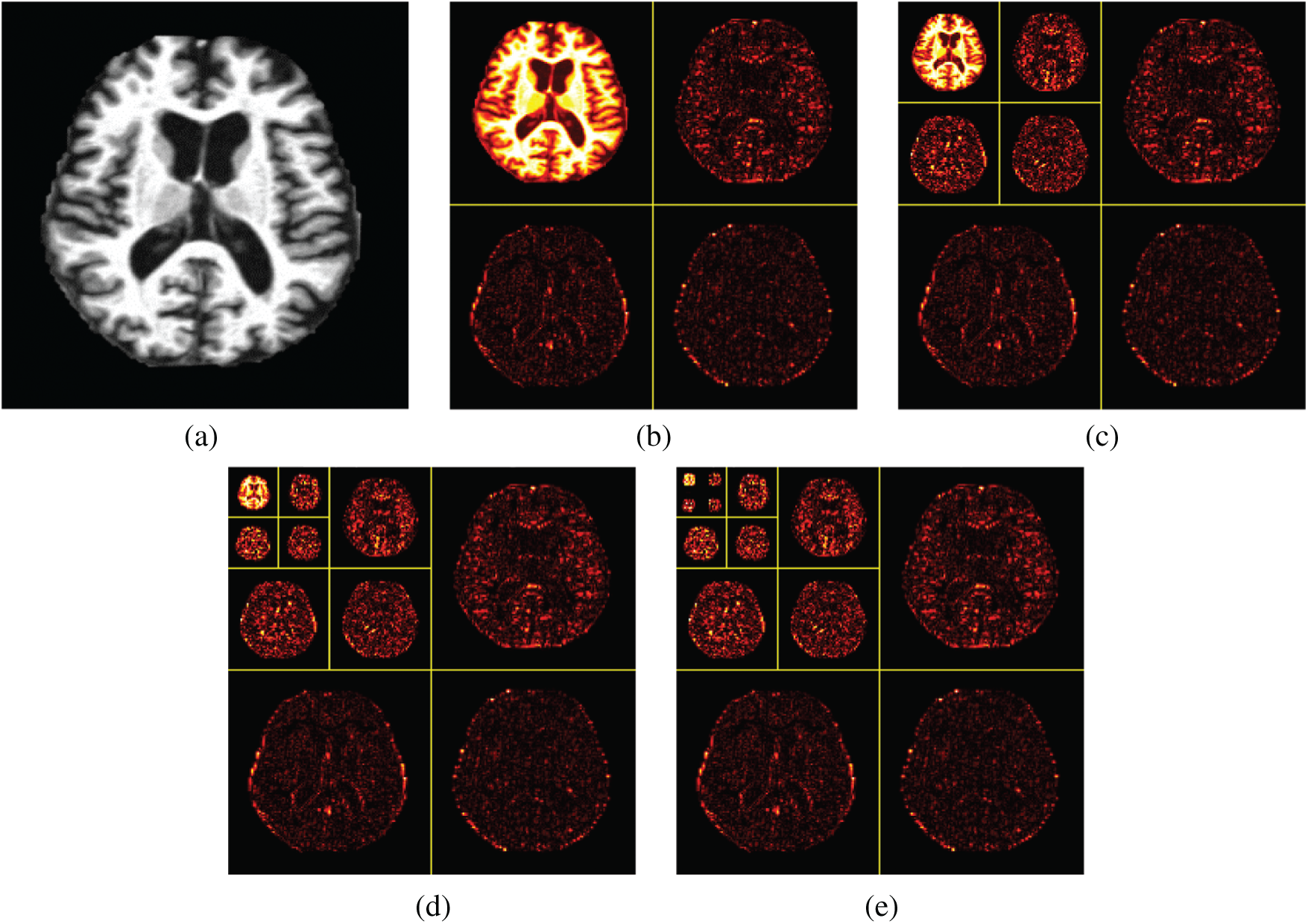
Figure 4: Wavelet decompositions. (a) Raw image (b) Level 1 decomposition (c) Level 2 decomposition (d) Level 3 decomposition (e) Level 4 decomposition
A Fourier coefficient usually represents a signal component that runs through the whole-time domain. The advantages of wavelet transform allow for more accurate local description and separation of signal features. For special signals, wavelet coefficients are suitable for most instantaneous signals, and it is easy to interpret image information. The advantage of wavelet transform is that its transform has not only the frequency-domain resolution of Fourier transform but also the time-domain or special resolution. However, because the one-dimensional signal is expressed by the two-dimensional coefficient, it is easy to have great redundancy.
3.2 Statistical Results of Different Decomposition Levels
Tab. 2 shows the performance of our model in each indicator after 10 runs of 10-fold cross-validation under the condition of decomposition Level 1. In the first experiment, we obtained the sensitive value of
Table 2: 10 runs of 10-fold cross-validation of our method (
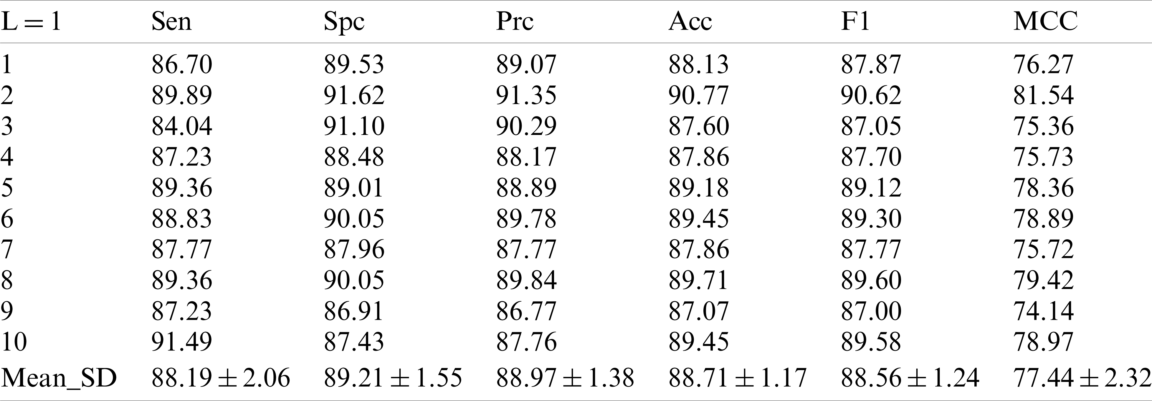
Compared with the existing methods support vector machine [6], pseudo Zernike moment [7] and Weighted fractional Fourier transform [8], it seems to improve in terms of value comparison, but this value has already been surpassed by other methods.
In the following experiments, the results of the experiments at the decomposition Level 2 are shown in Tab. 3. Sensitivity, specificity, precision, accuracy, F1 scores and MCC values were obtained as
Table 3: 10 runs of 10-fold cross-validation of our method (
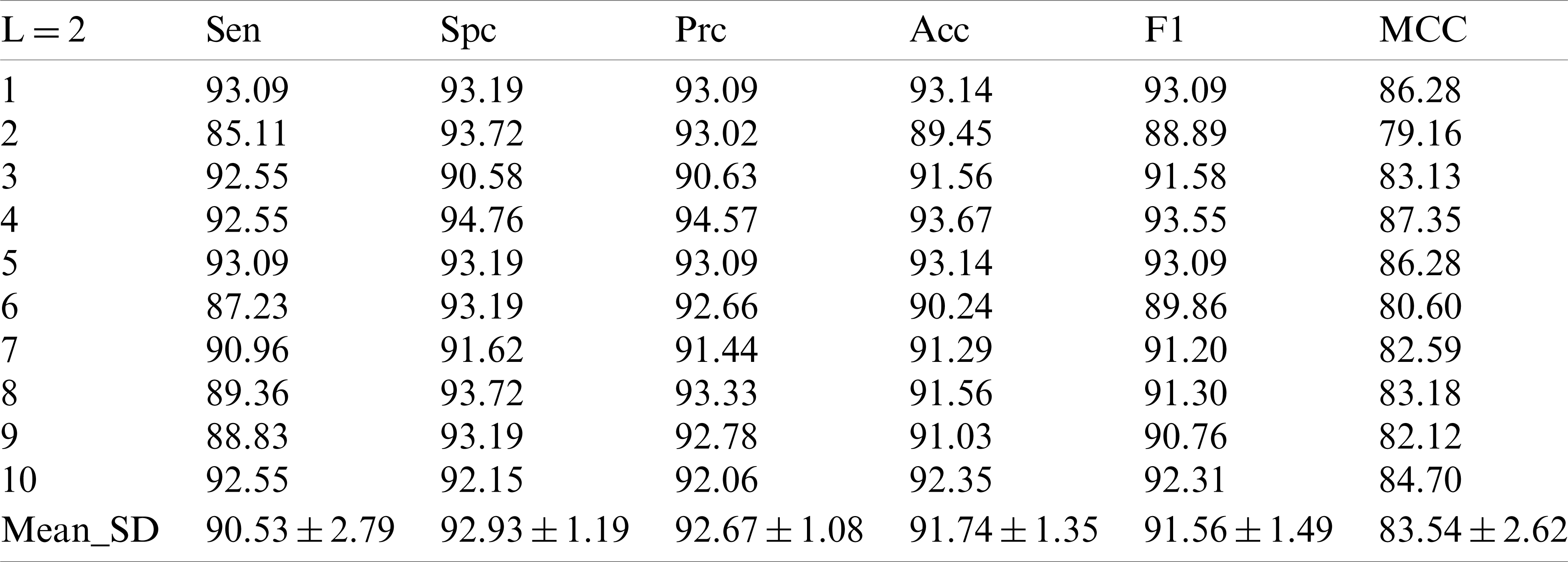
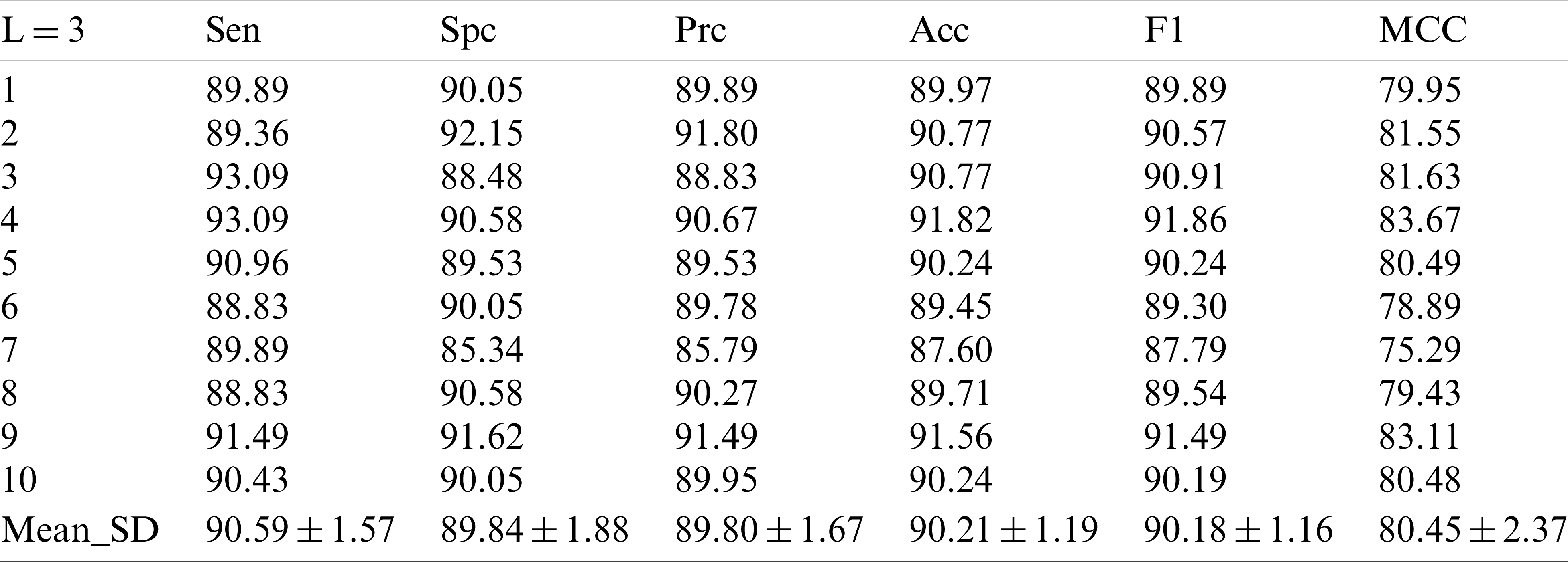
In the experiment with the decomposition Level 2, it can be seen that the improvement of the decomposition level is conducive to the improvement of the model test performance. In the decomposition Level 3 experiment in Tab. 4, we did obtain new and higher values, in which the sensor value is
Table 4: 10 runs of 10-fold cross-validation of our method (
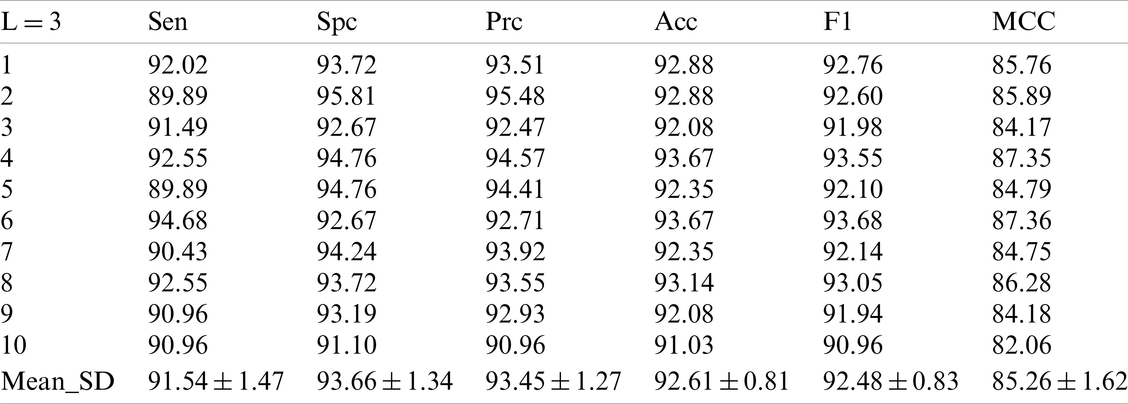
In the experiment with the decomposition Level 4 show in Tab. 5, there was no significant difference between the numerical value and the experiment with the decomposition Level 1, and the numerical value was even lower than that of the experiment with the decomposition Levels 2 and 3.
Table 5: 10 runs of 10-fold cross-validation of our method (
As can be seen from the Fig. 5, in the experiment before the decomposition Level 3, all values increase steadily. The value of MCC increases by leaps before decomposition Level 3, and drops to decomposition Level 4. However, the experimental performance evaluation value of decomposition Level 4 is generally lower than decomposition Level 2, the model performance drops sharply. Therefore, the optimal decomposition level in the experiment is 3, and the six evaluation results in the experiment are the highest value in the four experiments to obtain the best model performance.
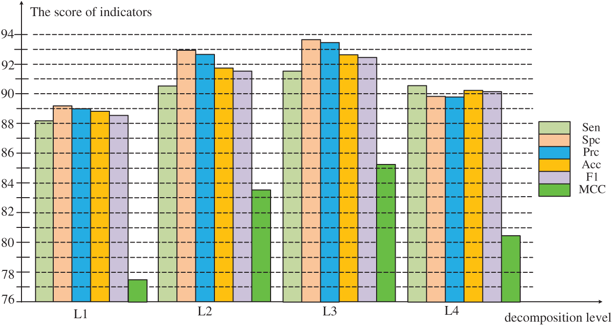
Figure 5: Comparison of evaluation results at different levels of decomposition
3.3 Comparison to State-of-the-Art
In this part, our method is compared with the most advanced methods in the field of image detection by combining wavelet energy entropy and linear regression classifier.
The first method uses Hu moment invariants to extract image features, and combines predator-prey adaptive inertia chaotic particle swarm optimization algorithm to train the single hidden layer neural network classifier [5]. It is shown in the form with the abbreviation of HMI-IPSO. The second method also takes Hu moment invariants as the image feature and combines two classifiers, twin support vector machine and generalized eigenvalue proximal support vector machine for detection [6]. In the table, this method is represented by SVM. The third method uses pseudo Zernike Moment and kernel support vector machine to conduct intelligent detection of images [7]. We describe this method in the table as PZM. The next method, we use WFFT for short, uses principal component analysis to extract the spectral features of weighted-type fractional Fourier transform and combines two variants of generalized eigenvalue proximal support vector machine and twin support vector machine similar to the second method for image classification [8]. The last comparison method uses wavelet entropy as image feature, and uses 2-layer feed-forward neural network and cat swarm optimization to search and track the image for identification.
The data for the comparison results of our methods and these methods are listed in Tab. 6, and Fig. 6 shows a bar chart of the comparison results.
Table 6: Comparison to state-of-the-art methods
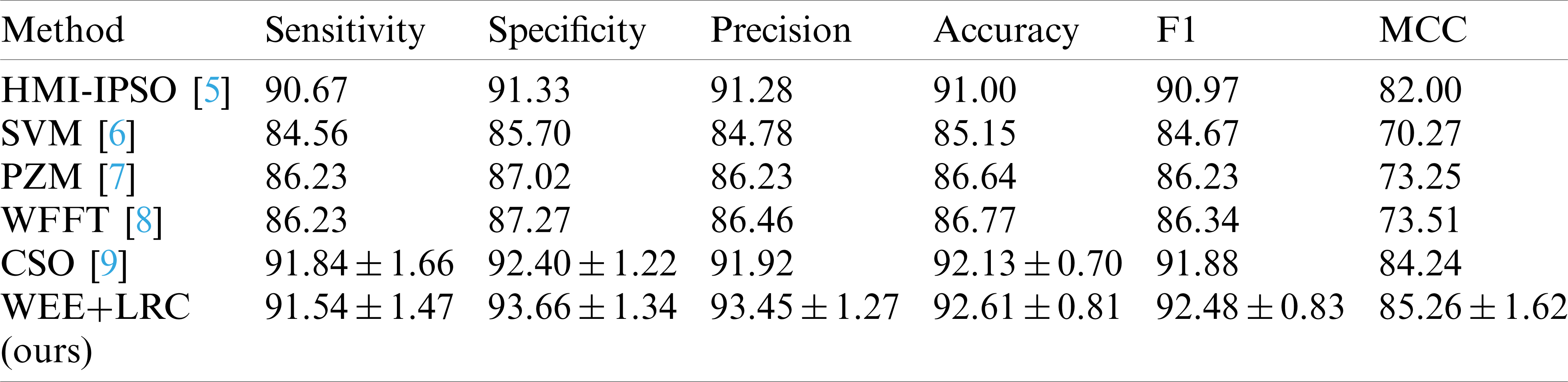
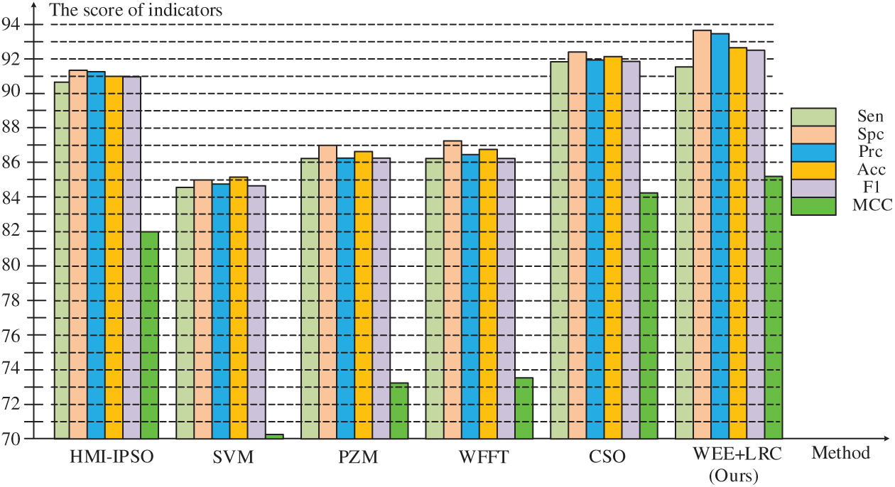
Figure 6: Comparison of six methods
It can be observed that the WEE+LRC method proposed by us achieved the best performance in all six evaluation values of the six methods. In the comparison of the specificity values of the six methods shown in the table, the SVM method obtained a score of 85.70%. PZM received a score of 87.02%. WFFT received a score of 87.27%. The HMI-IPSO method has been improved with a value of 91.33% Compared with the HMI-IPSO method, the CSO method increased to
In the precision comparison, SVM, PZM, WFFT, HMI-IPSO, CSO obtained 84.78%, 86.23%, 86.46%, 91.92%, 91.28%, respectively. Our WEE+LRC method was maintained at the highest score of
From the bar chart, our method maintained a high level of specificity, precision, accuracy, F1 score and Matthews correlation coefficient. Compared with the previous method, we have about 8% improvement in numerical values and a better score compared with the latest method, indicating that our algorithm has a higher performance.
We compared our feature extraction method with the popular wavelet energy and wavelet entropy. In order to ensure the fair comparison of the same conditions, we carried out three levels of the wavelet transform, and the comparison results are shown in Tab. 7. It can be seen that in the comparison of these six indicators, our approach is well beyond energy and entropy. In terms of sensitivity, specificity, precision, accuracy and F1 scores, our methods are almost above the wavelet energy and the wavelet entropy by about 1%–3%. In the Matthews coefficient comparison, it exceeds the other two methods by about 5%, 6%.
Table 7: WEE compared to wavelet energy and wavelet entropy (
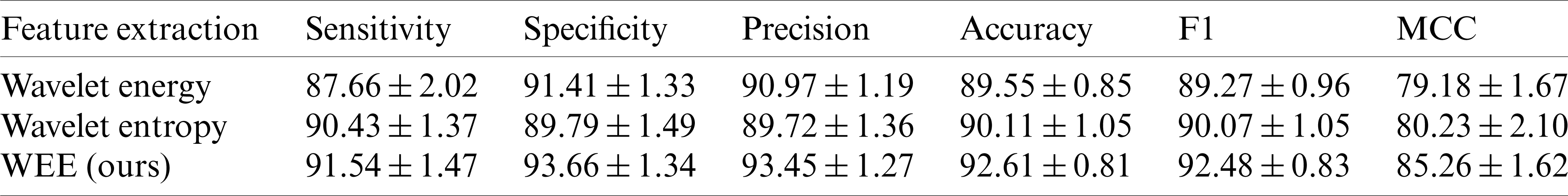
Fig. 7 below shows the difference between our approach and others more clearly than the table. In the comparison of sensitivity, accuracy and F1 scores, the highest scores of our method were
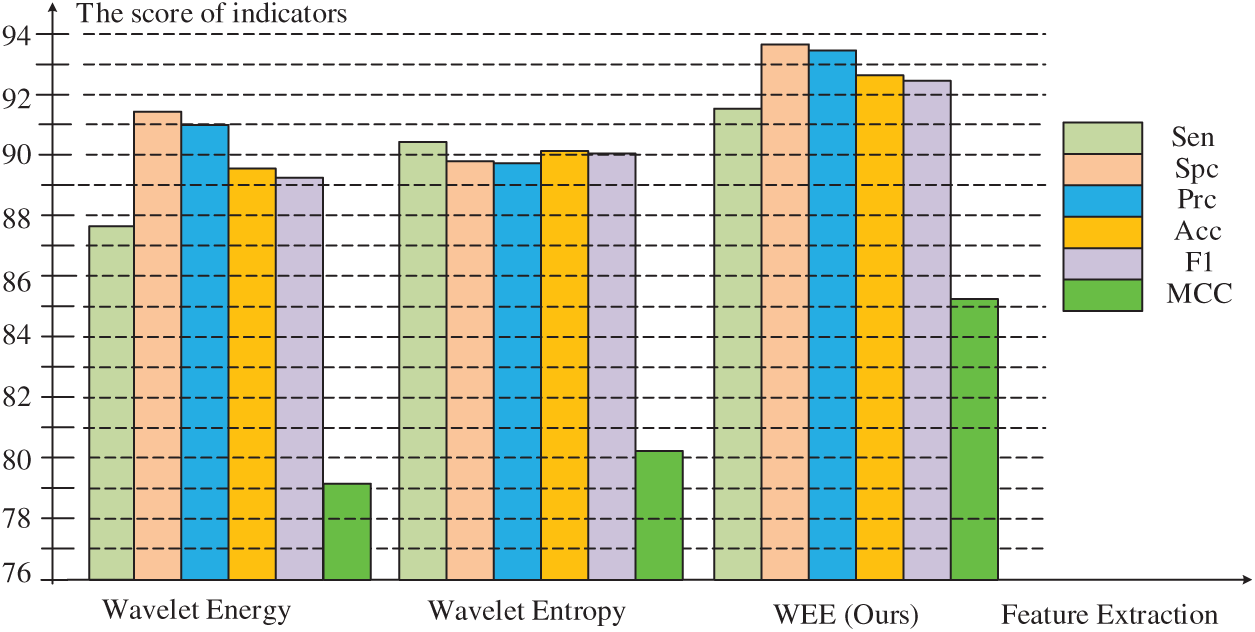
Figure 7: Comparison of three feature extraction methods
In the comparison of specificity and precision, although the wavelet energy fractions of
In the comparison of Matthews coefficient, it can be seen that there is a leap difference between our method and the other two methods. The highest value of our method is
In general, the score of the feature extraction method proposed by us is significantly better than that of wavelet energy and wavelet entropy in six evaluations, indicating that we have a feature extraction method with higher quality and higher precision to improve the overall performance of the model.
In this study, we compared our LRC classifier with different classifiers: Decision tree (DT), support vector machine (SVM), and naive Bayesian classifier (NBC). The results are shown in Tab. 8.
Table 8: Comparison with different classifiers
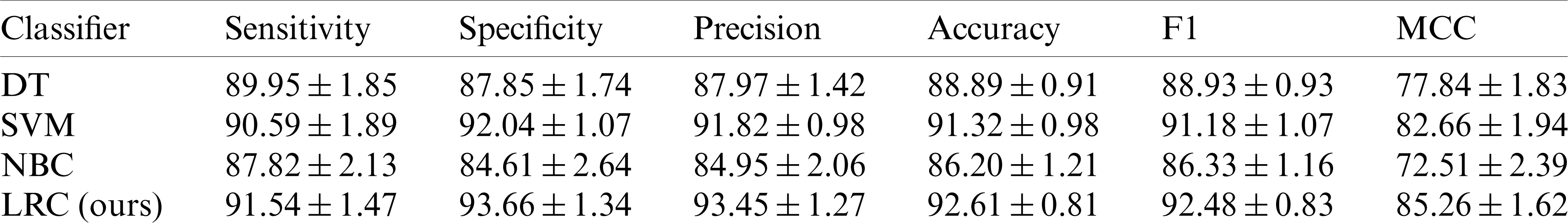
As can be seen from the data comparison of the table, the average value of our assessment is always the highest. In the comparison of six indicators, our method is stable above the SVM score by about 1%, and the DT method is lower than the SVM score by about 1% to 4% in all values. The approach of NBC had the lowest results in the experiment, at least 3% less than our approach. In particular, NBC’s approach was 12% lower than ours in the MCC comparison. Although the values of SVM are at least 1% and 4% higher than those of DT and NBC, respectively. The highest score of our method represents its best experimental performance among all method comparisons.
We propose a novel alcohol detection system, which is based on a new image extraction method wavelet energy entropy and uses linear regression classifier for diagnosis. Wavelet energy entropy extracted from magnetic resonance imaging (MRI) replaces image features with signals, which can simplify complex image information and thus improve detection efficiency. The linear regression classifier can visually distinguish and express the relationship between variables according to the image information provided. The experimental results of cross-validation show that the efficient modeling speed and running speed of linear regression classifier also have obvious advantages in comparison with the latest detection methods. For doctors, high quality and efficient auxiliary diagnostic tools are needed. Our proposed alcohol detection system can meet the diagnostic needs of doctors and help relieve their diagnostic pressure.
In future studies, our method can continuously improve performance, improve detection accuracy and reduce detection complexity through optimization experiments. The new study will not be limited to alcohol diagnosis, it could also be used for other types of classification tasks.
Funding Statement: This research was supported by Zhejiang Provincial Natural Science Foundation of China under Grant No. LY17F010003.
Conflicts of Interest: The authors declare that they have no conflicts of interest to report regarding the present study.
1. Viorreta, R. T., Gomez-Peinado, A., Quero-Palomino, V., Larumbe, S. M. (2020). Complications in chronic alcoholism: Extrapontine myelinolysis. European Psychiatry, 63, S633. [Google Scholar]
2. Sarraipo, V. S., Neto, F. S. L., de Carvalho, C. A. M., da Silva, J. P., Durand, M. T. et al. (2020). Expression of AIF, PARP, and miRNAs MIR-145, MIR-210, and MIR-486 associated with apoptosis in the corpus cavernosum of rats subjected to chronic alcoholism model. International Journal of Morphology, 38(6), 1639–1644. DOI 10.4067/S0717-95022020000601639. [Google Scholar] [CrossRef]
3. Mehla, V. K., Singhal, A., Singh, P. (2020). A novel approach for automated alcoholism detection using Fourier decomposition method. Journal of Neuroscience Methods, 346(3), 108945. DOI 10.1016/j.jneumeth.2020.108945. [Google Scholar] [CrossRef]
4. Gonzalez-Reimers, E., Romero-Acevedo, L., Espelosin-Ortega, E., Martin-Gonzalez, M. C., Quintero-Platt, G. et al. (2018). Soluble klotho and brain atrophy in alcoholism. Alcohol and Alcoholism, 53(5), 503–510. DOI 10.1093/alcalc/agy037. [Google Scholar] [CrossRef]
5. Hou, X. X. (2017). Alcoholism detection by medical robots based on Hu moment invariants and predator-prey adaptive-inertia chaotic particle swarm optimization. Computers and Electrical Engineering, 63, 126–138. DOI 10.1016/j.compeleceng.2017.08.021. [Google Scholar] [CrossRef]
6. Yang, J. (2017). Pathological brain detection in MRI scanning via Hu moment invariants and machine learning. Journal of Experimental & Theoretical Artificial Intelligence, 29(2), 299–312. DOI 10.1080/0952813X.2015.1132274. [Google Scholar] [CrossRef]
7. Jiang, Y. (2018). Exploring a smart pathological brain detection method on pseudo Zernike moment. Multimedia Tools and Applications, 77(17), 22589–22604. DOI 10.1007/s11042-017-4703-0. [Google Scholar] [CrossRef]
8. Chen, S., Yang, J. F., Phillips, P. (2015). Magnetic resonance brain image classification based on weighted-type fractional Fourier transform and nonparallel support vector machine. International Journal of Imaging Systems and Technology, 25(4), 317–327. DOI 10.1002/ima.22144. [Google Scholar] [CrossRef]
9. Qian, P. (2018). Cat swarm optimization applied to alcohol use disorder identification. Multimedia Tools and Applications, 77(17), 22875–22896. DOI 10.1007/s11042-018-6003-8. [Google Scholar] [CrossRef]
10. Sangaiah, A. K. (2020). Alcoholism identification via convolutional neural network based on parametric ReLU, dropout, and batch normalization. Neural Computing and Applications, 32, 665–680. DOI 10.1007/s00521-018-3924-0. [Google Scholar] [CrossRef]
11. Xie, S. (2019). Alcoholism identification based on an AlexNet transfer learning model. Frontiers in Psychiatry, 10, 205. DOI 10.3389/fpsyt.2019.00205. [Google Scholar] [CrossRef]
12. Shah, S., Sharma, M., Deb, D., Pachori, R. B. (2019). An automated alcoholism detection using orthogonal wavelet filter bank. Machine Intelligence and Signal Analysis, pp. 473–483. Singapore: Springer. [Google Scholar]
13. Bavkar, S., Iyer, B., Deosarkar, S. (2019). Detection of alcoholism: An EEG hybrid features and ensemble subspace K-NN based approach. Cham Distributed Computing and Internet Technology, pp. 161–168. Cham: Springer International Publishing. [Google Scholar]
14. Bavkar, S., Iyer, B., Deosarkar, S. (2020). BPSO based method for screening of alcoholism. Singapore ICCCE 2019, pp. 47–53. Singapore: Springer. [Google Scholar]
15. Duque, D., Garzon, J., Gharbi, T. (2020). A study of dispersion in chromatic confocal microscopy using digital image processing. Optics and Laser Technology, 131, 106414. DOI 10.1016/j.optlastec.2020.106414. [Google Scholar] [CrossRef]
16. Chadebecq, F., Vasconcelos, F., Mazomenos, E., Stoyanov, D. (2020). Computer vision in the surgical operating room. Visceral Medicine, 36(6), 456–462. DOI 10.1159/000511934. [Google Scholar] [CrossRef]
17. Bertolini, M., Besana, G. M., Notari, R., Turrini, C. (2020). Critical loci in computer vision and matrices dropping rank in codimension one. Journal of Pure and Applied Algebra, 224(12), 27. DOI 10.1016/j.jpaa.2020.106439. [Google Scholar] [CrossRef]
18. Manovich, L. (2021). Computer vision, human senses, and language of art. AI & Society, 8, DOI 10.1007/s00146-020-01094-9. [Google Scholar] [CrossRef]
19. Rasheed, A., Zafar, B., Rasheed, A., Ali, N., Sajid, M. et al. (2020). Fabric defect detection using computer vision techniques: A comprehensive review. Mathematical Problems in Engineering, 24(2), 8189403. DOI 10.1155/2020/8189403. [Google Scholar] [CrossRef]
20. Oliver, A. S., Anuradha, M., Justus, J. J., Bellam, K., Jayasankar, T. (2020). An efficient coding network based feature extraction with support vector machine based classification model for CT lung images. Journal of Medical Imaging and Health Informatics, 10(11), 2628–2633. DOI 10.1166/jmihi.2020.3263. [Google Scholar] [CrossRef]
21. Ramkumar, B., Laber, R., Bojinov, H., Hegde, R. S. (2020). GPU acceleration of the KAZE image feature extraction algorithm. Journal of Real-Time Image Processing, 17(5), 1169–1182. DOI 10.1007/s11554-019-00861-2. [Google Scholar] [CrossRef]
22. Dutta, S., Basu, B., Talukdar, F. A. (2021). Classification of lower limb activities based on discrete wavelet transform using on-body creeping wave propagation. IEEE Transactions on Instrumentation and Measurement, 70, 2502307. DOI 10.1109/tim.2020.3031210. [Google Scholar] [CrossRef]
23. Haq, E. U., Huang, J. J., Li, K., Ahmad, F., Banjerdpongchai, D. et al. (2020). Improved performance of detection and classification of 3-phase transmission line faults based on discrete wavelet transform and double-channel extreme learning machine. Electrical Engineering, 11, DOI 10.1007/s00202-020-01133-0. [Google Scholar] [CrossRef]
24. Khalid, M. J., Irfan, M., Ali, T., Gull, M., Draz, U. et al. (2020). Integration of discrete wavelet transform, DBSCAN, and classifiers for efficient content based image retrieval. Electronics, 9(11), 15. DOI 10.3390/electronics9111886. [Google Scholar] [CrossRef]
25. Khani, M. E., Winebrenner, D. P., Arbab, M. H. (2020). Phase function effects on identification of terahertz spectral signatures using the discrete wavelet transform. IEEE Transactions on Terahertz Science and Technology, 10(6), 656–666. DOI 10.1109/TTHZ.2020.2997595. [Google Scholar] [CrossRef]
26. Prabhakar, D. V. N., Kumar, M. S., Krishna, A. G. (2020). A novel hybrid transform approach with integration of fast fourier, discrete wavelet and discrete shearlet transforms for prediction of surface roughness on machined surfaces. Measurement, 164, 108011. DOI 10.1016/j.measurement.2020.108011. [Google Scholar] [CrossRef]
27. Dehestani, H., Ordokhani, Y., Razzaghi, M. (2021). Combination of Lucas wavelets with Legendre–Gauss quadrature for fractional Fredholm–Volterra integro-differential equations. Journal of Computational and Applied Mathematics, 382, 113070. DOI 10.1016/j.cam.2020.113070. [Google Scholar] [CrossRef]
28. Amin, R., Shah, K., Asif, M., Khan, I., Ullah, F. (2021). An efficient algorithm for numerical solution of fractional integro-differential equations via Haar wavelet. Journal of Computational and Applied Mathematics, 381, 113028. DOI 10.1016/j.cam.2020.113028. [Google Scholar] [CrossRef]
29. Martinez-Flores, C. (2021). Shannon entropy and Fisher information for endohedral confined one-and two-electron atoms. Physics Letters A, 386, 126988. DOI 10.1016/j.physleta.2020.126988. [Google Scholar] [CrossRef]
30. Kershenbaum, A., Demartsev, V., Gammon, D. E., Geffen, E., Gustison, M. L. et al. (2020). Shannon entropy as a robust estimator of Zipf’s Law in animal vocal communication repertoires. Methods in Ecology and Evolution, 1–12, DOI 10.1111/2041-210x.13536. [Google Scholar] [CrossRef]
31. Saha, S., Jose, J. (2020). Shannon entropy as an indicator of correlation and relativistic effects in confined atoms. Physical Review A, 102(5), 52824. DOI 10.1103/PhysRevA.102.052824. [Google Scholar] [CrossRef]
32. Vogel, E. E., Brevis, F. G., Pasten, D., Munoz, V., Miranda, R. A. et al. (2020). Measuring the seismic risk along the Nazca–South American subduction front: Shannon entropy and mutability. Natural Hazards and Earth System Sciences, 20(11), 2943–2960. DOI 10.5194/nhess-20-2943-2020. [Google Scholar] [CrossRef]
33. Prasad, D. V. V., Jaganathan, S. (2019). Null-space based facial classifier using linear regression and discriminant analysis method. Cluster Computing: The Journal of Networks Software Tools and Applications, 22, S9397–S9406. DOI 10.1007/s10586-018-2178-z. [Google Scholar] [CrossRef]
34. Naik, D. L., Kiran, R. (2018). Naive Bayes classifier, multivariate linear regression and experimental testing for classification and characterization of wheat straw based on mechanical properties. Industrial Crops and Products, 112, 434–448. DOI 10.1016/j.indcrop.2017.12.034. [Google Scholar] [CrossRef]
35. Vijh, S., Sarma, R., Kumar, S. (2021). Lung tumor segmentation using marker-controlled watershed and support vector machine. International Journal of E-Health and Medical Communications, 12(2), 51–64. DOI 10.4018/IJEHMC.2021030103. [Google Scholar] [CrossRef]
36. Mohammadi, M., Khorrami, M. K., Vatani, A., Ghasemzadeh, H., Vatanparast, H. et al. (2021). Genetic algorithm based support vector machine regression for prediction of SARA analysis in crude oil samples using ATR-FTIR spectroscopy. Spectrochimica Acta Part A: Molecular and Biomolecular Spectroscopy, 245(1), 118945. DOI 10.1016/j.saa.2020.118945. [Google Scholar] [CrossRef]
37. Sharma, N., Kolekar, M. H., Jha, K. (2021). EEG based dementia diagnosis using multi-class support vector machine with motor speed cognitive test. Biomedical Signal Processing and Control, 63, 102102. DOI 10.1016/j.bspc.2020.102102. [Google Scholar] [CrossRef]
38. Ban, M., Aliotta, L., Gigante, V., Mascha, E., Sola, A. et al. (2020). Distribution depth of stone consolidants applied on-site: Analytical modelling with field and lab cross-validation. Construction and Building Materials, 259, 120394. DOI 10.1016/j.conbuildmat.2020.120394. [Google Scholar] [CrossRef]
39. Kaminsky, A. L., Wang, Y., Pant, K. (2021). An efficient batch K-fold cross-validation voronoi adaptive sampling technique for global surrogate modeling. Journal of Mechanical Design, 143(1), 11706. DOI 10.1115/1.4047155. [Google Scholar] [CrossRef]
40. Fage, D., Deprez, G., Fontaine, B., Wolff, F., Cotton, F. (2021). Simultaneous determination of 8 beta-lactams and linezolid by an ultra-performance liquid chromatography method with UV detection and cross-validation with a commercial immunoassay for the quantification of linezolid. Talanta, 221, 121641. DOI 10.1016/j.talanta.2020.121641. [Google Scholar] [CrossRef]
41. Nakanishi-Ohno, Y., Yamasaki, Y. (2020). Multiplication method for fine-tuning regularization parameter of a sparse modeling technique tentatively optimized via cross validation. Journal of the Physical Society of Japan, 89(9), 94804. DOI 10.7566/JPSJ.89.094804. [Google Scholar] [CrossRef]
42. Jakštas, T., Balsevicius, T., Vaitkus, S., Padervinskis, E. (2020). Lithuanian version of nasolacrimal duct obstruction symptom scoring questionnaire: Cross-cultural adaptation and validation. Short- and long-term results. Clinical Otolaryngology, 45, 857–861. DOI 10.1111/coa.13606. [Google Scholar] [CrossRef]
43. Guttery, D. S. (2021). Improved breast cancer classification through combining graph convolutional network and convolutional neural network. Information Processing and Management, 58, 102439. DOI 10.1016/j.ipm.2020.102439. [Google Scholar] [CrossRef]
44. Wang, S. H. (2021). COVID-19 classification by CCSHNet with deep fusion using transfer learning and discriminant correlation analysis. Information Fusion, 68, 131–148. DOI 10.1016/j.inffus.2020.11.005. [Google Scholar] [CrossRef]
45. Satapathy, S. C. (2021). A five-layer deep convolutional neural network with stochastic pooling for chest CT-based COVID-19 diagnosis. Machine Vision and Applications, 32, 14. DOI 10.1007/s00138-020-01128. [Google Scholar] [CrossRef]
46. Satapathy, S. C., Wu, D. (2020). Improving ductal carcinoma in situ classification by convolutional neural network with exponential linear unit and rank-based weighted pooling. Complex & Intelligent Systems. 1–16. DOI 10.1007/s40747-020-00218-4. [Google Scholar] [CrossRef]
47. Pierazzi, F., Cristalli, S., Bruschi, D., Colajanni, M., Marchetti, M. et al. (2021). Glyph: Efficient ML-based detection of heap spraying attacks. IEEE Transactions on Information Forensics and Security, 16, 740–755. DOI 10.1109/TIFS.2020.3017925. [Google Scholar] [CrossRef]
48. Gaitonde, J. V., Lohani, R. B. (2020). Structural optimization and analysis of GaAs buried-gate OPFET for visible-light communication. Optical and Quantum Electronics, 52(12), 37. DOI 10.1007/s11082-020-02627-8. [Google Scholar] [CrossRef]
49. Das, S. R., Kaushal, A., Mandal, G., Trivedi, S. P. (2020). Bulk entanglement entropy and matrices. Journal of Physics A: Mathematical and Theoretical, 53(44), 444002. DOI 10.1088/1751-8121/abafe4. [Google Scholar] [CrossRef]
50. Duncan, M. J., Eyre, E. L. J., Cox, V., Roscoe, C. M. P., Faghy, M. A. et al. (2020). Cross-validation of Actigraph derived accelerometer cut-points for assessment of sedentary behaviour and physical activity in children aged 8–11 years. Acta Paediatrica, 109(9), 1825–1830. DOI 10.1111/apa.15189. [Google Scholar] [CrossRef]
 | This work is licensed under a Creative Commons Attribution 4.0 International License, which permits unrestricted use, distribution, and reproduction in any medium, provided the original work is properly cited. |