Computer Modeling in Engineering & Sciences

DOI: 10.32604/cmes.2021.012595

ARTICLE

Nonlinear Problems via a Convergence Accelerated Decomposition Method of Adomian

Mustafa Turkyilmazoglu1,2,*

1Department of Mathematics, Hacettepe University, Ankara, 06532, Turkey
2Department of Medical Research, China Medical University Hospital, China Medical University, Taichung, 40447, Taiwan
*Corresponding Author: Mustafa Turkyilmazoglu. Email: turkyilm@hacettepe.edu.tr
Received: 05 July 2020; Accepted: 12 November 2020

1  Introduction

Researchers prefer an easily accessible and user friendly method requiring less computational labor while accurately approximating highly nonlinear equations resulting from mathematical modeling of real-life phenomena. The Adomian decomposition method (ADM) is one such popular technique capable of dealing with the prevailing nonlinearities by means of Adomian polynomials [1,2]. A modification of the classical ADM is proposed within the current study based on the recent publications [3,4] successfully generating fast convergent ADM series solutions with as small Adomian polynomials as possible in the solution series.

A quick literature survey exhibits that ADM has been applied to many nonlinear equations [5]. To classify some of the recent bibliography, algebraic equations were contained within the references [6,7]. The ordinary differential equations were dealt within the citations [8–14]. The articles [15–18] covered the efforts to partial differential equations. Mathematical analysis of the convergence of ADM to certain nonlinear equations was fulfilled in the publications [19–21]. It can be successfully used to gain correct physical parameters domain [22]. A traffic model was also very recently treated in [23] via the Adomian method. The publications by [24,25] present investigation of some nonlinear problems via different numerical approaches.

It is now well-known that an inadequate arrangement of the classical ADM series may lead to non-convergent solutions or solutions with a poor convergence rate. To avoid these shortcomings, a parameter is generally inserted at the leading term of the Adomian series and later it is subtracted at the first order term not to break down the equation structure. This procedure was pursued by the recent publications [11,17,18]. However, how a proper value of the inserted parameter will be determined was not mentioned in these references. Instead, a randomly chosen value was assigned to it. A variety of modifications were also offered in the articles [26–31]. A successful formulation of the ADM was made in the recent work of [3] which was named as the optimal ADM. Further applications of the homotopy analytic approximate method may be found in the literature [32–35].

The motivation of the current work is, benefiting from the idea in [11], to devise a method that greatly improves the mathematical property of classical ADM. Within this aim, a reorganization of the ADM series is proposed by altering the early terms so that they incorporate extra controllable terms. The reason of such a treatment is to get a rapidly converging ADM solutions with the least Adomian polynomials. In place of randomly selecting, an optimum value of the introduced parameter is later determined through error on the grounds of total residual. With this value at our disposal, there is no doubt that the ADM method is convergent to the true solution in a most rapid way, not demanding a verification of the ADM solutions by numerical ones. The failure of the classical ADM in the usual form or in the Duan–Rach formulation is also prevented by a suitable value of the embedded parameter. The present approach can also extend the region of convergence of the traditional method. Examples of physical value are provided to justify and validate the given procedure.

2  Traditional Decomposition Method of Adomian

The usual steps of traditional ADM can be inferred from the aforementioned citations. The methodology in brief is such that under an invertible linear operator L and a forcing function f, it is desired to approximate the function u having the nonlinearity N(u) and satisfying the general nonlinear equation

L(u)=N(u)+f,(1)

with the initial and/or boundary restrictions

B(u)=b.(2)

Having inverted (1) under the restrictions (2) generally leads to

u=g+L-1[N(u)]+L-1[f],(3)

where g is due to the conditions in (2). If u is a single scalar parameter like (1) representing an algebraic equation, then there is no such g in (3), whereas, in the case of a variable u, L−1 denotes an integral operator giving rise to g in (3). Then (3) is a mixed Volterra-Fredholm type equation so-called as the Duan–Rach formulation in the recent literature, see for instance [13,14].

The subsequent series decompositions of u and N(u)

u=∑n=0∞un,N(u)=∑n=0∞An,(4)

in which An’s are the classical Adomian polynomials, are later substituted into (3). The solution u of (1) is finally generated from the recurrence relation

u0=g+L-1[f],un+1=L-1[An],n≥0.(5)

As a result, by means of the relations from (5), an approximate series solution of order M is obtained as

u=∑n=0Mun,(6)

which serves for practical purposes.

In general, the procedure in (5) yields convergent ADM series solutions, see for instance [19–21]. If not, to achieve convergent solutions or for computational conveniences some modifications in the terms ui in (5) are implemented as in the articles [11,12], without a proper mathematical evidence and support.

3  A Modified Decomposition Method of Adomian

To overcome the divergence of classical ADM or to speed up the convergence rate of the ADM series, the leading order term u0 in (5) (which is in compliance with the previous implementations, in for instance [11]) or some of the early terms, call ue, 0≤e≤Me, in (5) will be modified so that the modification will account for the change in the ADM by incorporating parameterized terms ũe(h) with h an embedded unknown parameter [3]. To exemplify, consider the modified version of (5) in the manner

u0=u0+ũ0(h),u1=u1+ũ1(h),⋮,ue=ue+ũe(h),⋮,un+1=L-1[An],n≥e.(7)

The following conditions for parameterized terms in the new algorithm (7) should be added

ũ0(0)=ũ1(0)=⋯=ũe(0)=0,(8)

so that it can be reduced to the traditional ADM for h = 0.

It is remarked that there is no a unique way of selecting the ũe(h) terms, but they must be as simple as possible in line with the simplicity inspiration of the ADM method itself. For instance, constants depending on h or simple power functions (or simple integrable functions) in combination with h can be used, refer to the illustrations belove for more details. We should remark that in the absence of tilde terms (or h) (7) dully conforms with (5). Having inserted such tilde terms in the modified ADM (7), the question now arises, how to determine the correct or proper value of h? So far, in ADM applications of this kind, only random or trial values are preassigned, see for instance [11] amongst others. On the other hand, we may either observe the least change in the plot of some physical quantities, the method is so-called as the constant h-level curves [36] giving rise to rough estimates for h, or we outline the following rigorous algorithm to determine the best or optimal h.

Algorithm. Consider the squared residual error corresponding to (1) defined by

Res(h)=∥L(u)-N(u)-f∥2,(9)

where either L2(Ω) or L(Ω) norms are employed. Moreover, u in (8) is owing to the modified ADM from (7). The optimum value of h is such that it minimizes the squared residual error (8) at the approximation level M.

As a consequence, the above Algorithm will generate the best value of h which will ensure the convergence of ADM series solution (7) in a fastest rate of convergence. The minimization task of (8) may be fulfilled by means of contemporary softwares, such as MAPPLE or MATHEMATICA.

4  Applications

Potential applications of the introduced ADM in (7) are given here. To control the error, we use the norm

err=∥ue-u(t)∥(10)

with the exact ue and ADM solution u.

4.1 An Algebraic Equation

As stated by Adomian [1] the classical ADM method (5) fails to result in a convergent solution of

u2-2u-2=0,(11)

for the solution u = −0.73205080757. On the other hand, when the new ADM is built via

u0=-1-h,u1=h+12u02,un+1=12∑k=0nukun-k,n≥1,(12)

Fig. 1 displays h-level curves at selected truncation orders M. The interval h∈(-0.35,-0.25) is observed to yield convergent ADM solutions, which excludes the traditional ADM with h = 0 [1].

Through the residual minimization

Res(h)=u2-2u-2(13)

at the approximation level M = 8, h = −0.2679492 is obtained as the optimum. The history and why this value is the best for the convergence control, as compared to the failure of classical ADM can be visualized in Tab. 1.

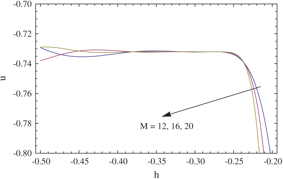
Figure 1: Convergence control parameter h regarding (11)

Table 1: Convergence of modified ADM (12) for Eq. (11) with different h. Paranthesis is for the absolute error (10)

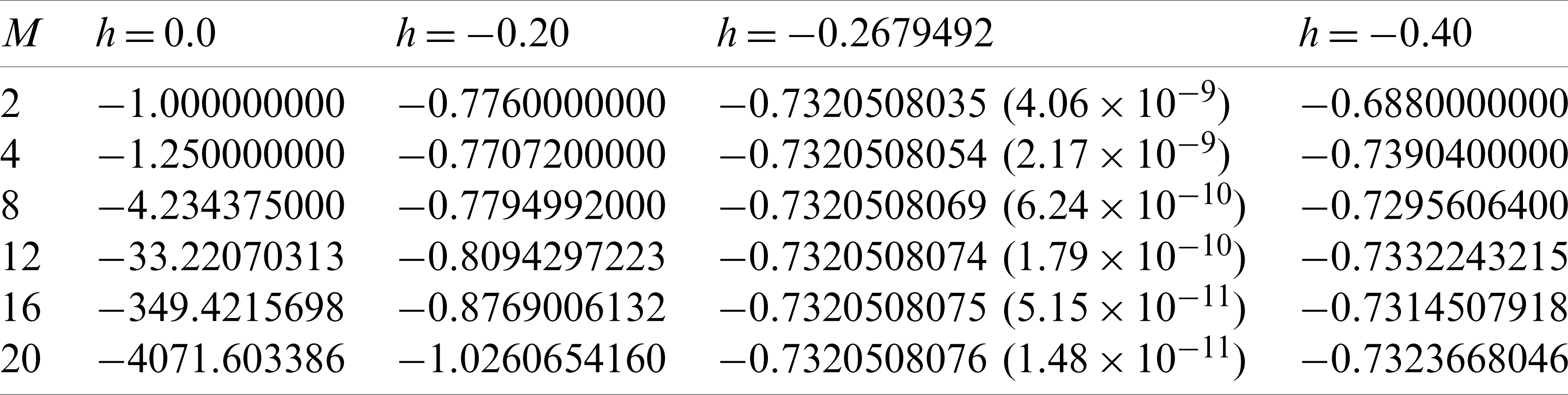
The convergent solution of (11) with the new modified ADM (12) at the approximation level M = 8 is found to be

u=1128(-542-6435h-37752h2-117348h3-210420h4-223594h5-140280h6-50292h7-9438h8-715h9),(14)

for which the optimum h is tabulated in Tab. 1.

4.2 Equation Involving Integral

Consider the equation given in [30]

u(η)=120(300+315η2+5η4+η6)-1150∫0η(η-τ)u(τ)2dτ,0≤η≤1.(15)

The modified ADM method (7) for the current integral problem is adopted as

u0(η)=120(300+315η2+5η4+η6)-hη2,u1(η)=hη2-1150∫0η(η-τ)u0(τ)2dτ,un+1(η)=-1150∫0η(η-τ)∑k=0nuk(τ)un-k(τ)dτ,n≥1.(16)

We find h∈(-1500,1500) for the convergence interval in Fig. 2, refer also to [3]. A comparison and convergence accelerating feature of the present ADM can be visualized from the Tab. 2. It is noticed from Tab. 2 that even the 4th-order modified ADM (16) is able to produce the solution accurate of order 10−10, which is adequate in practical purposes.

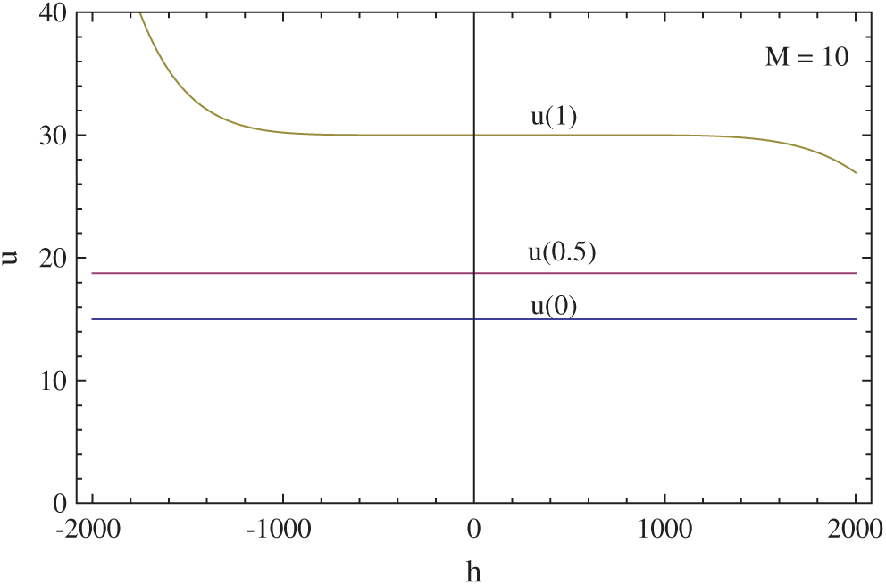
Figure 2: Convergence control parameter h regarding (15)

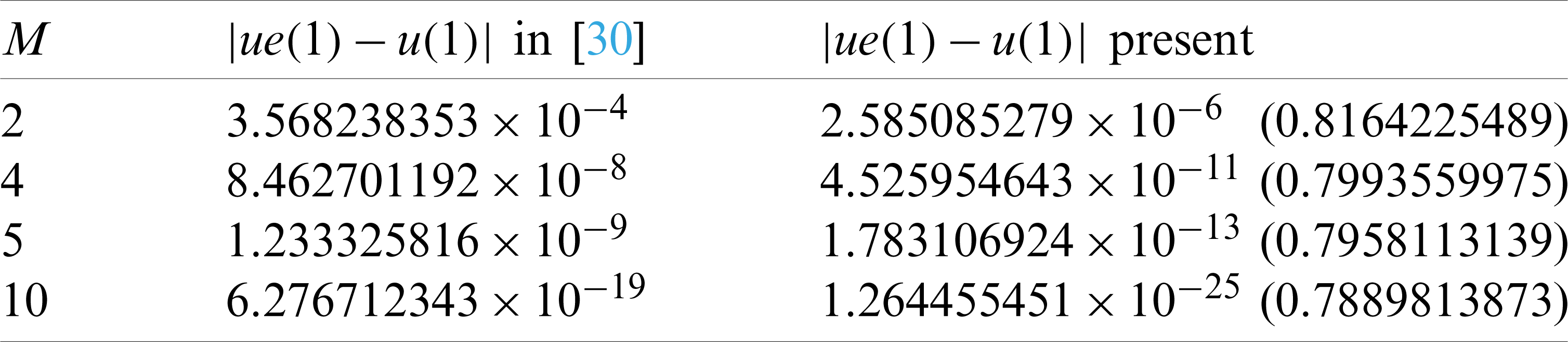
Table 2: Errors in (15) regarding (14). Parenthesis denotes the optimum values of h

4.3 A Fin with Porosity Feature

As taken from [14], a porous fin can be modelled via

u′′=su2+β2u,0<η<1,u′(0)=0,u(1)=1.(17)

In (17), temperature along the fin is u, and s and β are physical parameters.

The modified ADM algorithm (7) here is

u0(η)=θ0-hη2,u1(η)=hη2+∫0η∫0η(su0(η)2+β2u0(η))dηdη,un+1(η)=∫0η∫0η(β2un(η)+s∑k=0nuk(η)un-k(η))dηdη,n≥1.(18)

At the selected values s = 5 and β=1, the history of convergence is tabulated in Tab. 3. It is seen how useful the modified ADM over the classical one by more than doubling the convergence rate at the same number of iterations. The CPU times evaluated by MATHEMATICA through the residual are shown in Tab. 3. The list proves the improved efficiency of the current method over the classical ADM.

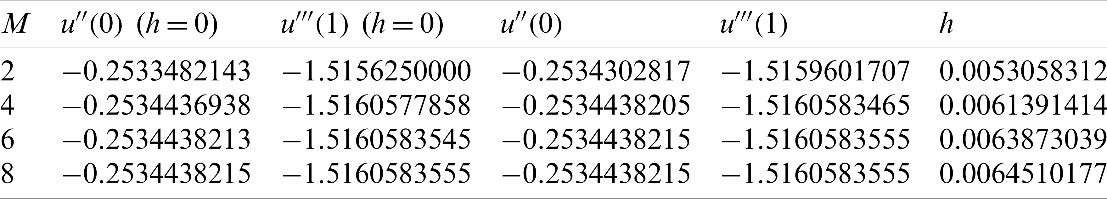
Table 3: Residual errors of classical ADM and modified ADM (18) for Eq. (17) with s = 5 and β=1. Parenthesis denote the optimum values of h

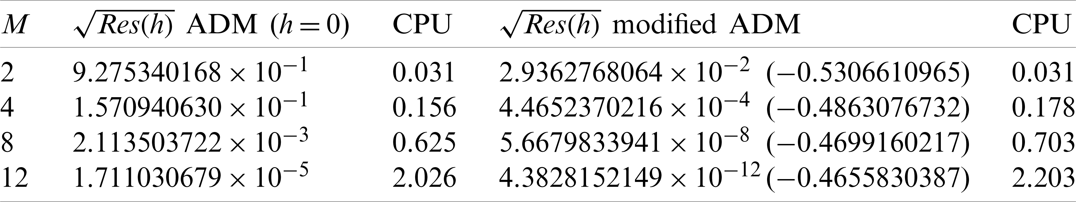
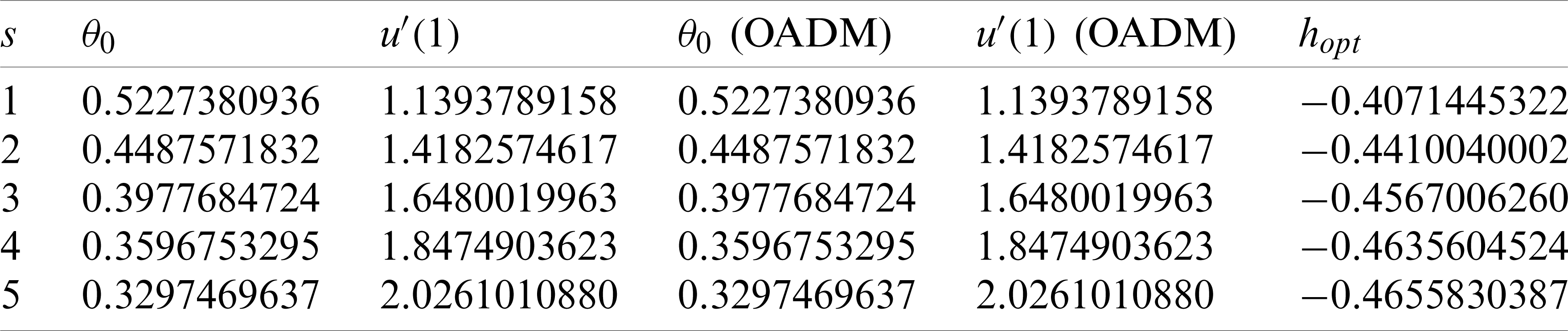
The values of u(0) and u′(1) are listed in Tab. 4 with M = 12 from the ADM and also with the optimums hopt. The ADM (18) excellently compares with the full numerical solutions and hence, they can be used without consulting a numerical verification.

Table 4: Numerical and modified ADM results regarding (17) [3]

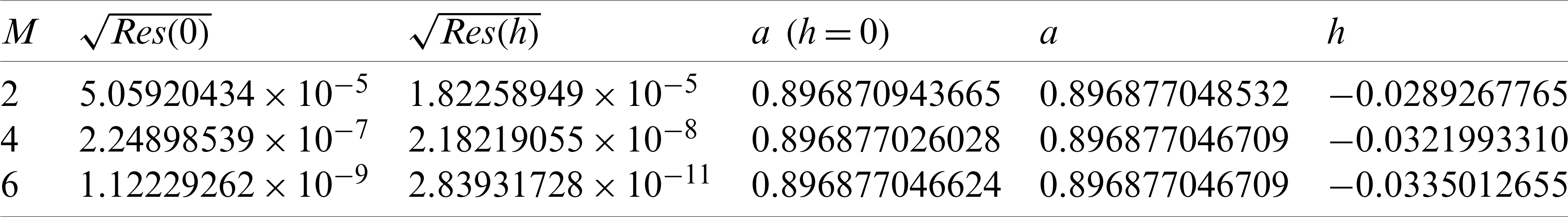
Instead of the modification of ADM in (18), we may use the Duan–Rach formulation involving no unknown parameters within it except the embedded parameter h

u0(η)=1-h,u1(η)=h+∫1η∫0η(su0(η)2+β2u0(η))dηdη,un+1(η)=∫1η∫0η(β2un(η)+s∑k=0nuk(η)un-k(η))dηdη,n≥1.(19)

Choosing s=β=1, Fig. 3 shows h −level curves, indicating that the prescription of h must be made within the range (0.39, 0.49) to ensure the convergence of the modified ADM 19. The exact values of u(0) and u′(1) are respectively, 0.522738093570 and 1.13937891581.

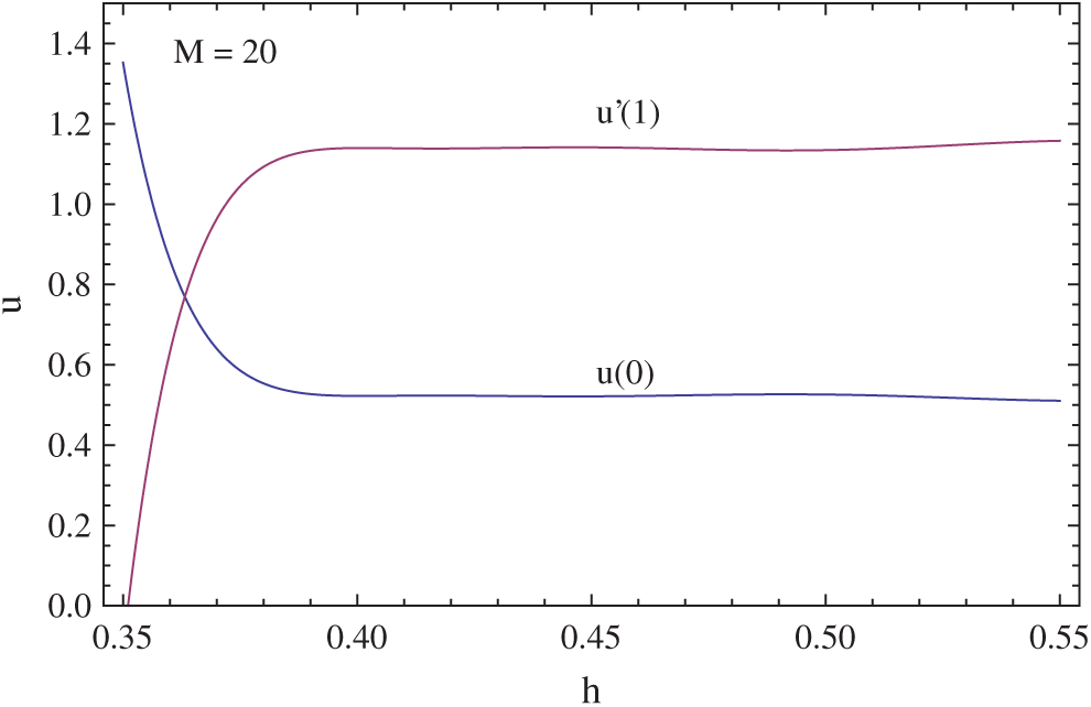
Figure 3: Convergence control parameter h regarding (17)

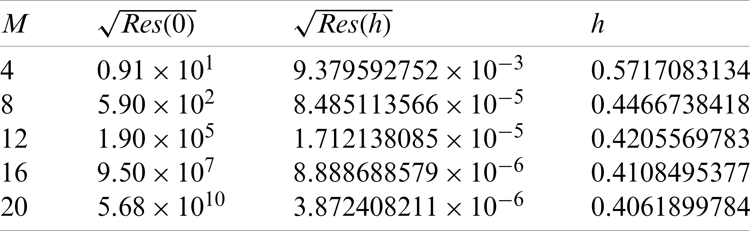
To demonstrate the power of the modified ADM (19), Tab. 5 shows the squared residual error (9) from both the novel and classical ADM. It is unfortunate to observe that the Duan–Rach formulation (19) with h = 0 fails to converge, however, the optimum embedded parameter h insures that the modified ADM is convergent for the present physical problem, even if the convergence is not as fast as the modified formulation in (18).

Table 5: Values of Res(h) for (17) from the classical and modified ADM methods

4.4 Gelfand Equation

The Gelfand equation [5] involves exponential nonlinearity [8]

u′′=eu,u(η=0)=u(η=1)=0,(20)

with u′(0)=-0.4636325917 [3].

In line with the publications [5,8] when h = 0, the modified ADM is

u0(η)=0,u1(η)=-h-η2+η22,u2(η)=h-(-124-h2)η-hη22-η312+η424,un+1(η)=-η∫01∫0ηAndηdη+∫0η∫0ηAndηdη,n≥2,(21)

where An(h,η) are the polynomials of Adomian for eu(η), encompassing all boundary conditions in (20) within the Duan–Rach approach, and we have

u′(0)=-∫01∫0ηAndηdη.

Fig. 4 shows the predicted convergence control parameters. With M = 12, an optimum value for the embedding parameter h is found to be −0.01274 from the Algorithm in (9). We find that the residual error is 1.6835117258×10-15 with u′(0)=-0.4636325917 from the present approach. On the other hand, and error of 4.813740934×10-9 with u′(0)=-0.4636325899 is calculated from the traditional ADM. Our value is given by

u′(0)=-7670935983223893726911654529071288638504960+15169262547373h37157048852152320000+7945655577131h2243290200817664000+9908796519071h38536498274304000+17536069217h4980755776000+38157057179h5373621248000+10097225749h657480192000+93183637h71045094400+1216277h881285120+147689h9174182400+283h1021772800+h1179833600.(22)

The success of the present modified ADM (21) is thus obvious.

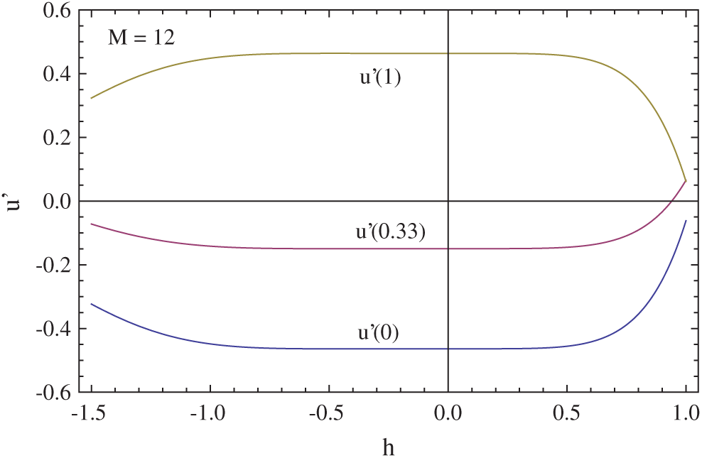
Figure 4: Convergence control parameter h regarding (20)

4.5 Electrostatic Cantilever Micro-Electromechanical System

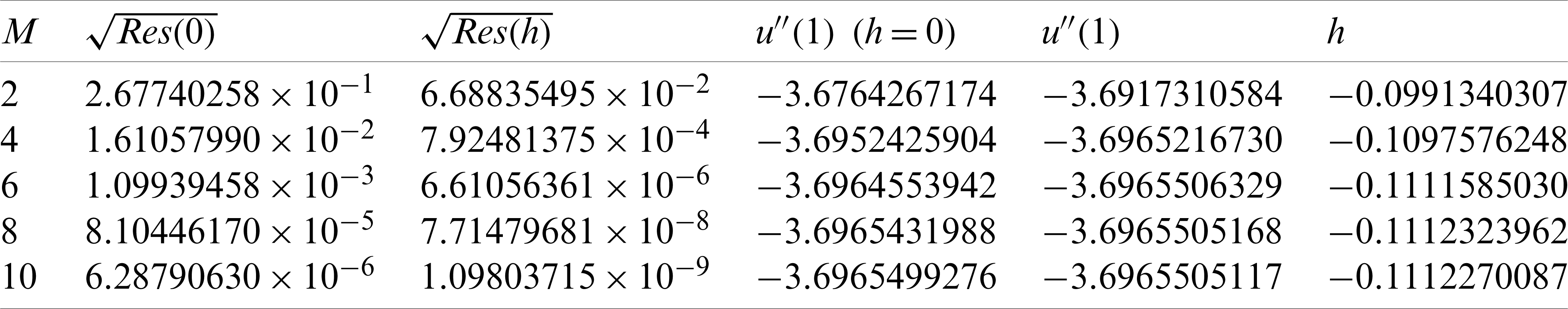
The beam-type electrostatic actuators for the nonlinear cantilever micro-electro mechanical systems are modelled by the fourth-order boundary value problem from [11]

u′′′′=-αKuK-βu2-γu,0<η<1,K=3,4,u(0)=1,u′(0)=u′′(1)=u′′′(1)=0.(23)

To comply with the Duan–Rach Adomian decomposition method in [11], the present modified ADM is

u0(η)=1-h,u1(η)=h+∫0η∫0η∫1η∫1ηA0dηdηdηdη=h+(αK+β-hβ+(-1+h)2γ)η2(6+(-4+η)η)24(-1+h)3,un+1(η)=∫0η∫0η∫1η∫1ηAndηdηdηdηn≥1,(24)

where the Adomian polynomials An(h,η) are due to the negative-power nonlinearities in (23), see [11] for more details.

For the fixed parameters K = 3, αK=0.2, β=0.5 and γ=0.25, Fig. 5 produced from (24) helps us guess the proper values of embedded parameter h. Small values of h are seen to be adequate to get convergent ADM solutions.

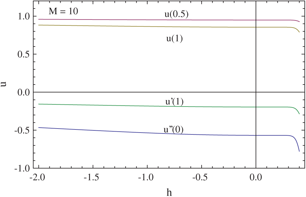
Figure 5: Convergence control parameter h regarding (23)

Fig. 6 demonstrates different approximation levels M, and it signifies to h = 0.1045421730 as the optimum h when M = 10. With this optimum value of the embedding parameter, the squared residual error for the current problem is Res=3.2727623195×10-9, whereas the classical residual error with h = 0 is Res=8.7520447833×10-5. This implies that much more Adomian series terms are required for the classical ADM to reach the accuracy of the modified ADM here. Moreover, from [11] the physical values are u′′(0)=-0.56764 and u′′′(0)=1.07585 evaluated with 12 Adomian polynomials. The present values are u′′(0)=-0.5676684138 and u′′′(0)=1.0758898885 evaluated with only 10 Adomian polynomials, correct to 9 decimal places. Hence, the advantage of the present modification is clear for the present highly nonlinear physical problem. We should remark that with the present Algorithm, the validation of the ADM results against the numerical ones is no longer a prerequisite. Also, there is no need to evaluate error remainder functions, nor to consult to Pade-approximates to increase the accuracy, both of which as implemented in [11].

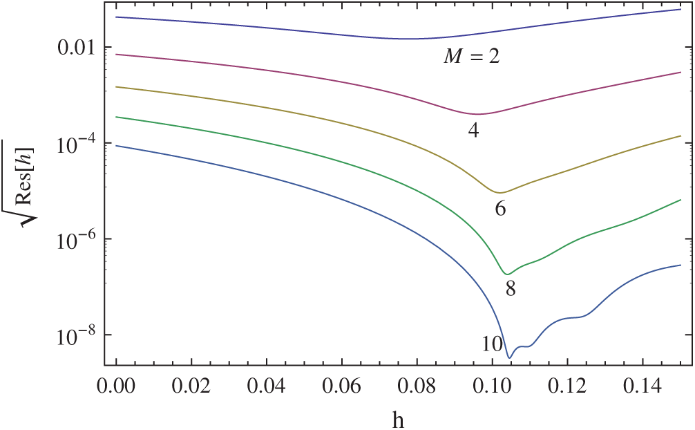
Figure 6: Error regarding (23) for various M

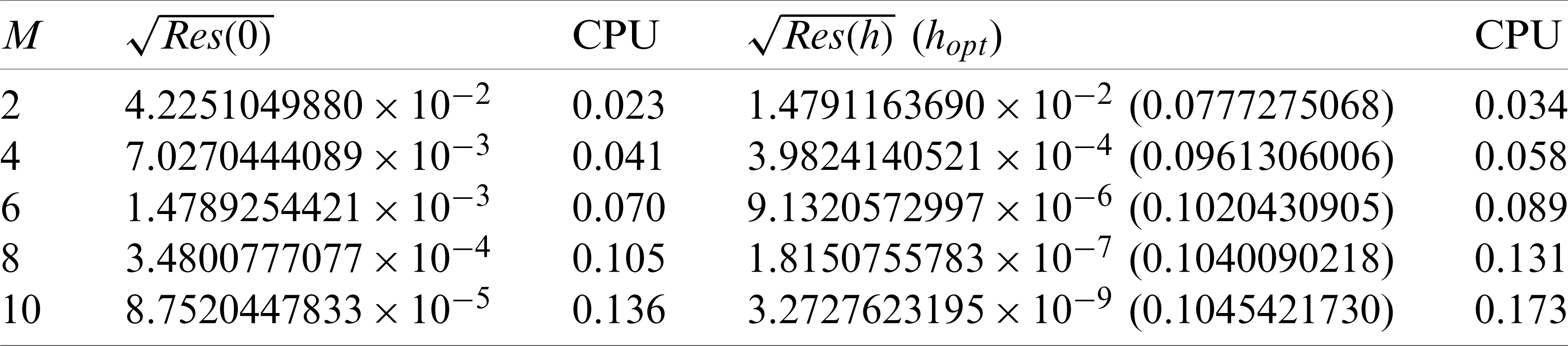
The convergence accelerating feature of the present modified ADM (24) as compared to the classical ADM is better visualized from the Tab. 6. Table also shows the comparable CPU times.

Table 6: Convergence history of modified ADM vs. classical ADM for Eq. (23)

4.6 Electrostatic Cantilever Nano-Electromechanical System

Nonlinear model for the electrostatic double cantilever nano-electromechanical system in the case of Casimir force (K = 4) is given by [11]

u′′′′=-αKuK-βu2-γu,0<η<1,u(0)=u(1)=1,u′(0)=u′(1)=0.(25)

We adopt the subsequent modified ADM, that conforms to the classical ADM (h = 0) given in [15]

u0(η)=1-h,u1(η)=h+(2η3-3η2)∫01∫0η∫0η∫0ηA0dηdηdηdη+(η2-η3)∫01∫0η∫0ηA0dηdηdη+∫0η∫0η∫0η∫0ηA0dηdηdηdη=h-(αK+(-1+h)2(β+γ-hγ))(-1+η)2η224(-1+h)4,un+1(η)=(2η3-3η2)∫01∫0η∫0η∫0ηAndηdηdηdη+(η2-η3)∫01∫0η∫0ηAndηdηdη+∫0η∫0η∫0η∫0ηAndηdηdηdη,n≥1,(26)

where the Adomian polynomials An(h,η) are due to the negative-power nonlinearities in (25), see [11] for more details.

For the specific parameters αK=1, β=1.5 and γ=0.5, Fig. 7 displays the constant h-level curves drawn at the approximation level M = 8. Similar to the previous example, very small values of h are seen to be adequate to get convergent ADM.

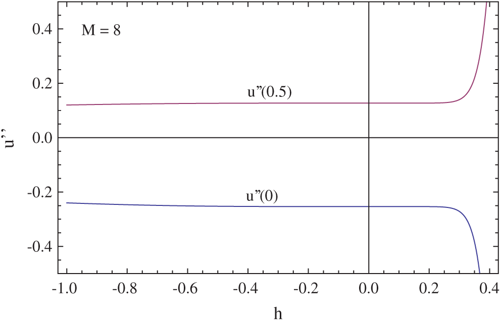
Figure 7: Convergence control parameter h regarding (25)

In order to evaluate the performance of modified ADM over the classical one, Tab. 7 shows the unknown physical quantities u′′(0)=u′′(1) and u′′′(1) at several truncation orders M. The faster convergence rate of the present ADM is apparent.

Table 7: Values of u′′(0) and u′′′(1) for (25) from the classical and modified ADM methods

To illustrate, the analytical formula computed via the present algorithm (26) at M = 4 for the value of u′′(0) is given by

u′′(0)=133476463820800(-1+h)19(8484398647110-161202053045835h+1450626144581925h2-8210561431139865h3+32657066457192189h4-96557260487752602h5+219137184603173574h6-389199830265020934h7+547311661233315516h8-613303909999850619h9+548763779900139189h10-391219305253946049h11+220658166826273313h12-97137704049404928h13+32601652101188352h14-8015172092928000h15+1344650417510400h16-133905855283200h17+5579410636800h18),(27)

which is of almost nine degree of accuracy as seen from Tab. 7.

4.7 Lane–Emden Equation

We consider the Lane–Emden type boundary value problem from [9]

u′′+kxu′-rus+u=0,0<x<1,u′(0)=0,5u(1)+u′(1)=5,(28)

that models the oxygen diffusion in a spherical cell with Michaelis–Menten uptake kinetics. We take into account the subsequent constants to comply with the literature [9]

k=4,r=0.76129,s=0.03119.

The modified ADM that is offered for the present problem is then

u0(η)=a-h,u1(η)=h+76129(a-h)η210(3119+100000a-100000h),un+1(η)=13∫0ηt(1-(tη)3)Andt,n≥1,(29)

which conforms with the classical ADM of [9] in the limit h→0 and the Adomian polynomials An(h,η) are to account for the nonlinearity rus+u. The interest is to determine the physical value of u(0) = a.

We present Tab. 8 to demonstrate the performance of the modified ADM (29) versus the classical ADM. The expected practical accuracy is met at lower Adomian series approximations via the modified method.

Table 8: Values of u(0) = a and Res(h) for (28) from the classical and modified ADM methods

4.8 The Fluid Flow of Jeffery–Hamel

The Jeffery–Hamel fluid flow problem is modelled via [22]

u′′′+2αReuu′+(4-Ha)α2u′=0,0<η<1,u(0)=1,u′(0)=u(1)=0,(30)

with α, Re and Ha are the physical parameters [13].

Following the successful Duan–Rach ADM formulation of the problem (30) in [17], we propose the following modified version

u0(η)=1-η2-h,u1(η)=-160αη2(-1+η2)(5(-4+Ha)α+2Re(-4+η2))+16h(6-Reαη2(-1+η2)),un+1(η)=-η2∫01∫0η∫0ηAndηdηdη+∫0η∫0η∫0ηAndηdηdη,n≥1,(31)

where An(h,η)=-(4-Ha)α2un′(η)-2αRe∑k=0nuk(η)un-k′(η) are the Adomian polynomials.

For the diverging channel, considering the specific parameters α=50, Re = 50 and Ha = 1000 to be in line with [13], the constant h-level curves are depicted in Fig. 8 at the approximation order M = 8. Accordingly, we expect the convergency of the modified ADM (31) in the vicinity of zero.

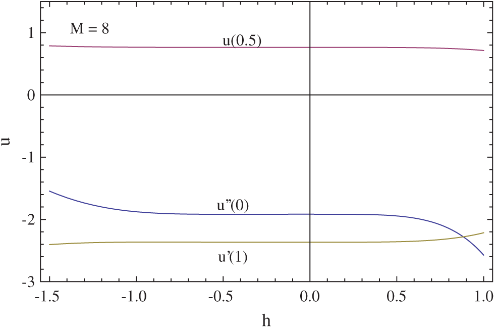
Figure 8: Convergence control parameter h regarding (30)

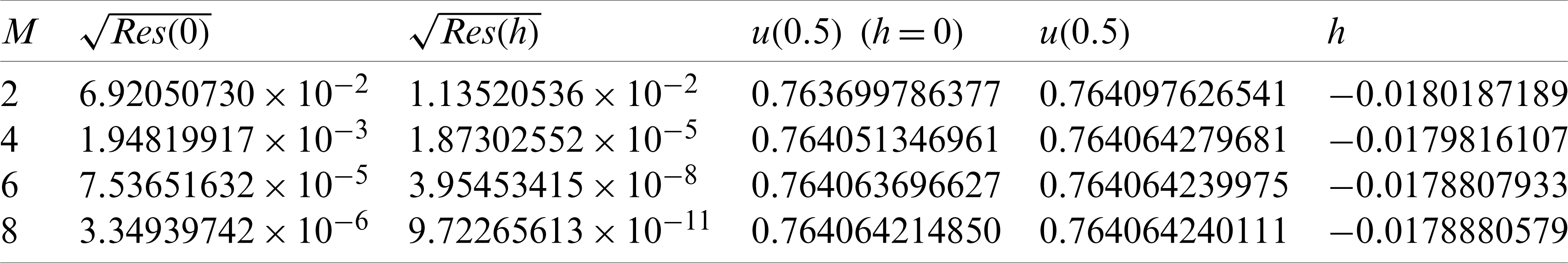
The performance of modified ADM (31) is next measured by computing the centerline velocity u(0.5) (numerical value is 0.764064240111) at different approximation levels M as shown in Tab. 9. It is observed that 10 digits of accuracy is quickly reached by the present ADM, whereas the classical ADM falls behind. Hence, even though it was not clearly mentioned in [13] (see Tab. 1 therein), the accuracy of order 10−8 as obtained via the classical ADM demands at least 15–20 Adomian polynomials, whereas only 6 Adomian polynomials are sufficient to gain the same accuracy with the present modification.

Table 9: Values of u(0.5) and Res(h) for (30) from the classical and modified ADM methods

4.9 Squeezing Two Parallel Plates

The flow squeezed between two parallel plates are modelled by the nonlinear equations [22]

u(4)-SA(1-ϕ)2.5(ηu′′′+3u′′+u′u′′-uu′′′)=0,0<η<1,u(0)=u′′(0)=0,u(1)=1,u′(1)=0,(32)

see [14] for the flow parameters.

In accordance with the Duan–Rach ADM formulation of the physical problem (32) in [14], we set the modified ADM in the form

u0(η)=12(3η-η3)-hη3,u1(η)=1560(560hη3+A(-27+2h)(1+2h)Sη(-3+η2)(1-ϕ)2.5+2A(1+2h)Sη5(-28+(1+2h)η2)(1-ϕ)5/2+14A(-192+h)(1+2h)S(η-η3)(1-ϕ)2.5),

un+1(η)=12(η-η3)∫01∫0η∫0ηAndηdηdη+12(η3-3η)∫01∫0η∫0η∫0ηAndηdηdηdη+∫0η∫0η∫0η∫0ηAndηdηdηdη,(33)

where

An(h,η)=SA(1-ϕ)2.5(ηun′′′(η)+3un′′(η)+∑k=0n(uk′(η)un-k′′(η)-uk(η)un-k′′′(η))) are the Adomian polynomials.

To make a comparison with the classical ADM in [14], we set the parameters S = 1, ϕ=0.02 and concentrate on Cu-Water nanofluid with ρs=8933 and ρf=997.1. The corresponding constant h-level curves are plotted in Fig. 9. It appears that the convergence of the modified ADM (32) is guaranteed if h is selected in the overlapping interval (-1,1).

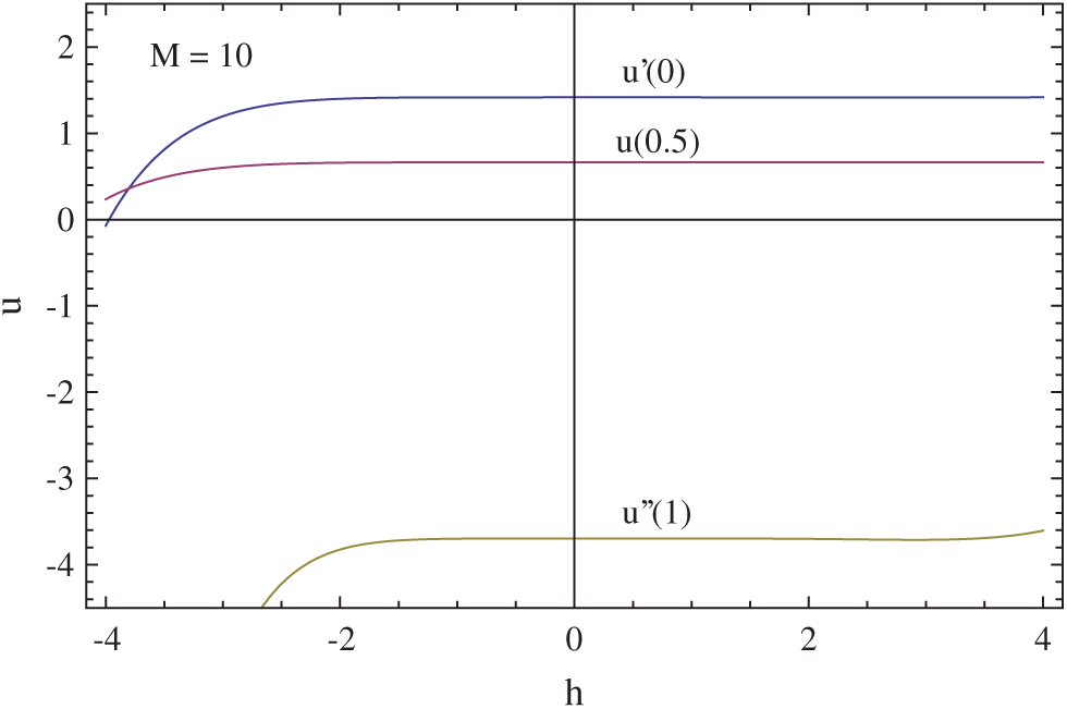
Figure 9: Convergence control parameter h regarding (32)

The effects of iterative number M on the skin friction u′′(1) are next demonstrated in Tab. 10. The advantage of the modified ADM (33) with optimum values of embedding parameter h is clearly observed against the classical ADM with h = 0. It appears that the accuracy of classical ADM of O(10−8) as displayed in Tab. 2 of [18] clearly requires more Adomian series terms (see M = 8 in Tab. 10) as compared to the less terms needed in the modified ADM here.

Table 10: Values of u′′(1) and Res(h) for (32) from the classical and modified ADM methods

The following fourth-order modified ADM series solution for the skin friction may serve good to the purpose of engineering applications if not high accuracy is required

u′′(1)=12940824761875(-8822474285625-2100589115625AS(1-ϕ)5/2-53295A3(1036330+h2(1966073+36h(-77288+16563h)))S3(1-ϕ)15/2-72747675A2(3687+1468h3)S2(-1+ϕ)5+A4(1+2h)(12606590933+h(-17941167514+h(12710854094-4619738103h+509582226h2)))S4(-1+ϕ)10).(34)

4.10 Nonlinear Oscillator Problem

Let us consider the nonlinear oscillator Duffing problem (see [36] (Chapter 5) and [4])

u′′+u+u3=0,u(0)=1,u′(0)=0;0≤t≤3,(35)

which involves a cubic nonlinearity.

The improved ADM can be given via

u0(t)=1-ht,u1(t)=ht-∫0t∫0t(un-1(t)+A0(t))dtdt,un+1(t)=-∫0t∫0tAn(t)dtdt,n≥1,(36)

with the Adomian terms An(t) in (35).

The classical Adomian method with h = 0 in (36) is not convergent, whereas with h = 0.68981924, the residual error becomes Res(h)=0.02589439, and the convergency is satisfied as revealed in Fig. 10 for the domain of definition.

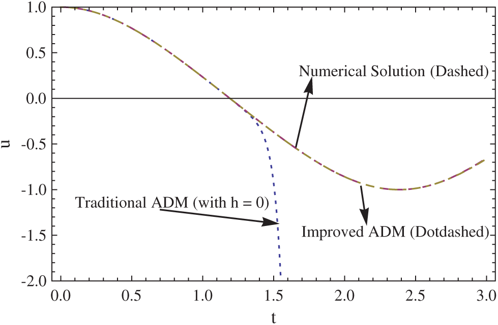
Figure 10: Convergence control parameter h regarding (35)

4.11 Diffusion Equation

Let us consider the nonlinear diffusion equation, see [18] and [3]

ut+u+u3=(u2ux)x,u(x,0)=ex3,0≤x≤1,0≤t≤1,(37)

for which [18] presents an exact solution.

The form of modified ADM for the partial differential equation (37) is

u0(x,t)=ex3(1-ht),u1(x,t)=12ex3t(-2+h(2+t)),un+1(x,t)=∫0tAn(h,x,t)dt,n≥1,(38)

where

An(h,x,t) are the Adomian polynomials corresponding to the function − u − u3+(u2ux)x.

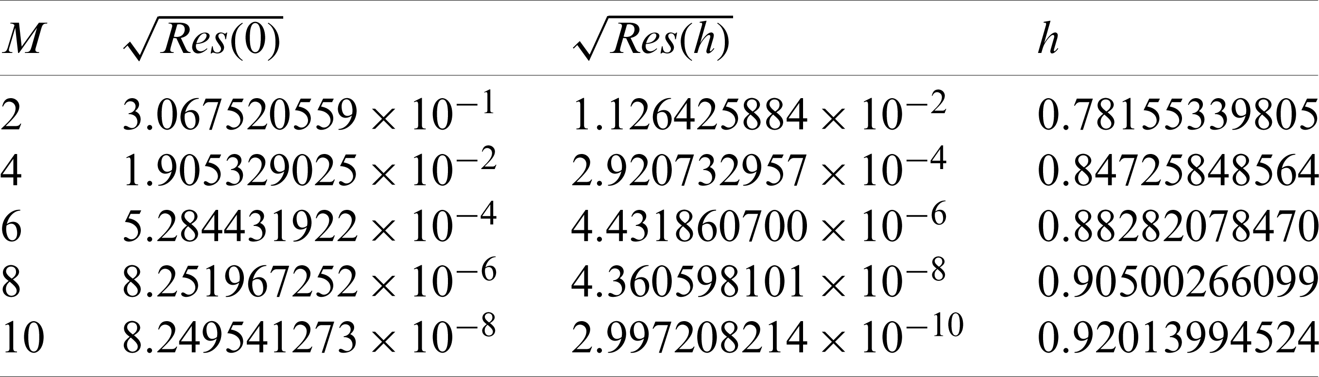
Fig. 11 shows the constant h-level curves at the approximation level M = 10, indicating a very large range of embedding parameter h.

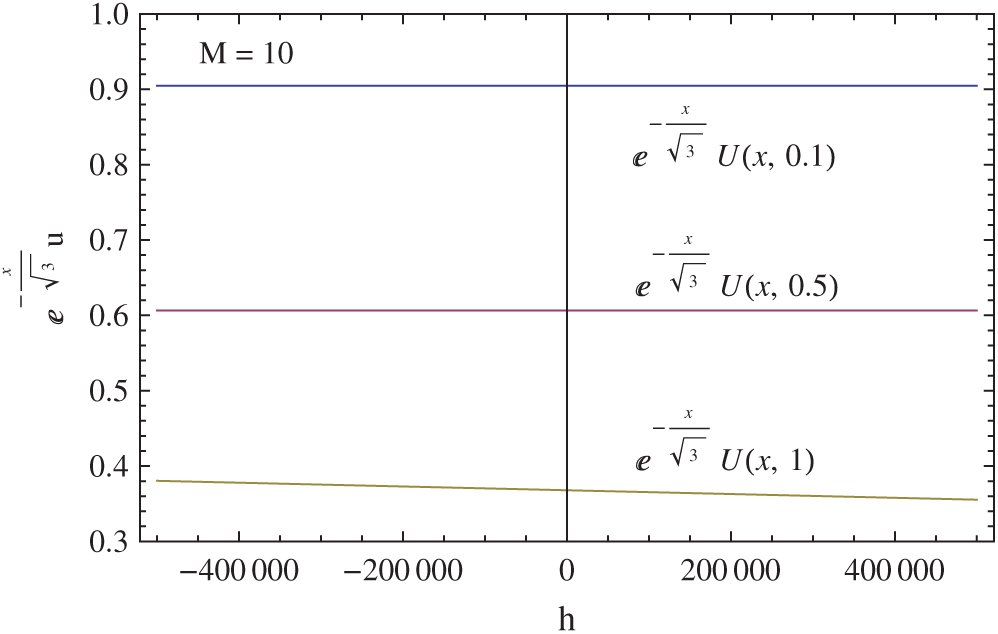
Figure 11: Convergence control parameter h regarding (37)

Actually at this truncation of the modified ADM series, it is obtained

u(x,t)=ex3(-ht1111!+∑n=010(-1)ntnn!).(39)

Defining the squared residual error for (37) as

Res(h)=||ut+u+u3-(u2ux)x||2=∫01∫01(ut+u+u3-(u2ux)x)2dxdt,(40)

Tab. 11 tabulates how the modified ADM has smaller residual errors.

Table 11: The residual errors Res(h) for (37) from the classical and modified ADM methods

4.12 Burger’s Equation

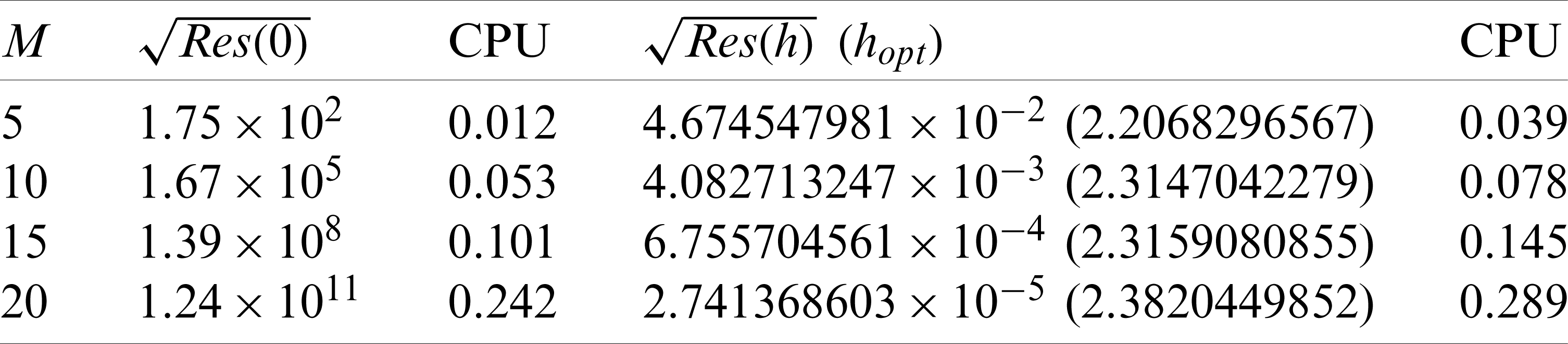
The final example is known as Burger’s equation [3]

ut+uux=uxx,u(x,0)=2x,0≤x≤1,0≤t≤1,(41)

with an exact solution u(x,t)=2x1+2t.

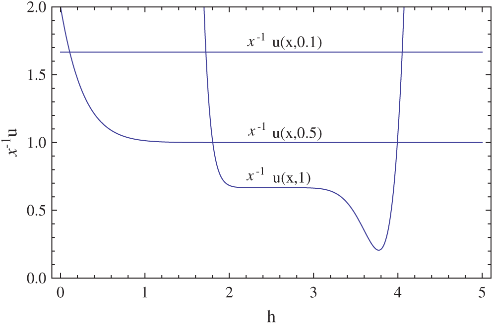
Figure 12: Convergence control parameter h regarding (41)

The form of modified ADM for the partial differential equation (40) is

u0(x,t)=x(2-ht),u1(x,t)=-13t(12+h(-3+t(-6+ht)))x,un+1(x,t)=∫0tAn(h,x,t)dt,n≥1,(42)

where

An(h,x,t) are the Adomian polynomials corresponding to the function uxx − uux.

The traditional ADM with h = 0 in the domain 0≤x≤1,0≤t≤1 is noticed to fail to produce a convergent series as also clear in Fig. 12, because h = 0 is not lying in the overlapping region.

With the definition

Res(h)=||ut+uux-uxx||2=∫01∫01(ut+uux-uxx)2dxdt,(43)

Tab. 12 justifies the success of the present modified ADM over the classical divergent one, both in terms of accuracy and computational cost.

Table 12: The residual errors Res(h) for (41) from the classical and modified ADM methods

5  Concluding Remarks

The aim of the present work is to present superiority over the well-known Adomian decomposition method (ADM) often employed in the recent literature to analytically approximate solutions to highly nonlinear algebraic and differential equations of some real physical motions. Within this aim, a reformulation of the ADM is targeted to prevent first the failure and then convergence acceleration of the classical Adomian polynomials.

To accomplish the objective, the classical ADM is modified by inserting some simple parameterized terms into the early iterates involving an embedded parameter to control and pacing the convergence of the generated ADM series. In order to determine the best suitable value or the optimum value of this parameter, squared residual minimizing of the governing equation is proposed. This enables us to overcome the divergence of the classical ADM, and more importantly, there is no need to check out the results against the numerical ones, as usually has to be done in traditional ADM studies, since the optimum embedded parameter obtained is an insurance for ADM series convergence in a most rapid manner.

Physical examples selected from the recent application of ADM demonstrate the validity, accuracy and power of the present approach in terms of generating the convergent solution within the least number of iterations. In particular, the Duan-Rach modification of the ADM incorporating all the boundaries mostly used in the recent ADM applications takes great benefit of the present proposal, otherwise there is always the inevitable danger that it may lead to non physical solutions. The present approach successfully extends the convergence interval of the studied problem. In conclusion, the present formulation of ADM offers a promising tool to treat more strongly nonlinear equations/systems of real life phenomena.

Funding Statement: The author received no specific funding for this study.

Conflicts of Interest: The author declares that he has no conflicts of interest to report regarding the present study.

This work is licensed under a Creative Commons Attribution 4.0 International License, which permits unrestricted use, distribution, and reproduction in any medium, provided the original work is properly cited.