Computer Modeling in Engineering & Sciences

DOI: 10.32604/cmes.2021.013603

ARTICLE

Spectral Solutions of Linear and Nonlinear BVPs Using Certain Jacobi Polynomials Generalizing Third- and Fourth-Kinds of Chebyshev Polynomials

W. M. Abd-Elhameed1,2,*and Asmaa M. Alkenedri2

1Department of Mathematics, Faculty of Science, Cairo University, Giza, Egypt
2Department of Mathematics, College of Science, University of Jeddah, Jeddah, Saudi Arabia
*Corresponding Author: W. M. Abd-Elhameed. Email: walee_9@yahoo.com
Received: 12 August 2020; Accepted: 26 November 2020

1  Introduction

It is well-known that the Chebyshev polynomials play vital roles in the scope of mathematical analysis and its applications. The first- and second-kinds are special symmetric polynomials of the Jacobi polynomials, so they are ultraspherical polynomials. These two kinds of Chebyshev polynomials are the most popular kinds, and they are employed extensively in numerical analysis, see for example [1–4]. There are other four kinds of Chebyshev polynomials. Third- and fourth-kinds are also special kinds of Jacobi polynomials, but they differ from the first- and second-kinds since they are not ultraspherical polynomials. In fact, they are non-symmetric Jacobi polynomials with certain parameters. There are considerable publications devoted to investigating these kinds of polynomials from both theoretical and practical points of view. For some articles in this direction, one can be referred to [5–7]. Fifth- and sixth-kinds of Chebyshev polynomials are not special cases of the Jacobi polynomials. These polynomials were first established by Jamei in his Ph.D. dissertation [8]. Recently, these kinds of polynomials have been employed for treating numerically some types of differential equations, see [9–11].

Spectral methods are essential in numerical analysis. These methods have been utilized fruitfully for obtaining numerical solutions of various kinds of differential and integral equations. The philosophy in the application of spectral methods is based on writing the desired numerical solution in terms of certain “basis functions,” which may be expressed as combinations of various orthogonal polynomials. There are three celebrated spectral methods; they are tau, collocation, and Galerkin methods. Galerkin method is based on choosing suitable combinations of orthogonal polynomials satisfying the underlying boundary/initial conditions [12]. Tau method is more flexible than the Galerkin method due to the freedom in choosing the basis functions. Collocation method is the most popular method because of its capability to treat all kinds of differential equations. There are considerable contributions employ this method in different types of differential equations [13–15]. For a survey on spectral methods and their applications, one can consult [16–21].

The problems of establishing derivatives and integrals formulas of different orthogonal polynomials in terms of their original polynomials are of great interest. These formulas play important parts in obtaining spectral solutions of various differential equations. For example, the authors in [5,6] derived explicit formulas of the high-order derivatives and repeated integrals of Chebyshev polynomials of third- and fourth-kinds, and after that, they utilized the derived formulas for obtaining spectral solutions of some boundary value problems (BVPs).

Boundary value problems have important roles due to their appearance in almost all branches related to applied sciences such as engineering, fluid mechanics, and optimization theory (see, [22]). Some examples concerning applications of BVPs are given with details in [22]. Moreover, the author showed that, at some times, it is more appropriate to transform high-order BVPs into systems of differential equations. Many real-life phenomena can be described by high-order BVPs.

Regarding the even-order BVPs, they arise in numerous problems. The free vibrations analysis of beam structures is governed by a fourth-order ordinary differential equation [23]. The vibration behavior of a ring structures is governed by a sixth-order ordinary differential equation [24]. Eighth-order BVPs arise in torsional vibration of uniform beams [25]. In addition, 10th- and 12th-orders appear in applications. When a uniform magnetic field is applied across the fluid in the same direction as gravity. Ordinary convection and overstability yield a 10th-order and a 12th-order BVPs, respectively [26]. For applications regarding the high-order BVPs appear in hydrodynamic and hydromagnetic stability, fluid dynamics, astronomy, beam and long wave theory [27,28]. For some other applications of these kinds of problems, one can be referred to [29–31].

Several studies were performed for the numerical solutions of these types of equations. Some of the algorithms treat these kinds are the perturbation and homotopy perturbation methods in [32], differential transform methods in [26] and spectral methods in [15,33–37].

The main objectives of this article can be summarized in the following items:

Deriving high-order derivatives formulas of certain classes of polynomials that generalize Chebyshev polynomials of the third- and fourth-kinds.

Implementing and analyzing an algorithm for the numerical solutions of even-order linear BVPs based on the application of the spectral Galerkin method.

Introducing a collocation algorithm for treating both linear and nonlinear BVPs.

The current paper is organized as follows. In Section 2, we give some relevant properties of Jacobi polynomials. In Section 3, we derive in detail two new formulas which give explicitly the high-order derivatives of Jacobi polynomials whose parameters difference is one. In Section 4, we present a spectral Galerkin algorithm for solving some high even-order linear BVPs with constant coefficients. Section 5 is devoted to presenting another algorithm for treating linear and nonlinear BVPs based on the application of a suitable collocation algorithm. Section 6 is interested in solving the connection problem between certain Jacobi polynomials and the Legendre polynomials. In Section 7, we investigate the convergence and error analysis of the proposed expansion in Section 5. In Section 8, we present some numerical examples including comparisons with some other methods to ascertain the accuracy and efficiency of the proposed algorithms presented in Sections 4 and 5. Finally, some conclusions are reported in Section 9.

2  Some Fundamental Properties of Jacobi Polynomials

The classical Jacobi polynomials , is a polynomial of degree m which can be defined in hypergeometric form as

where

It is easy to see the following special values

It is desirable to define the normalized orthogonal Jacobi polynomials as [38]

which gives . We have the following six special cases of the normalized Jacobi polynomials.

where , Tm(x), Um(x), Vm(x), Wm(x) and Pm(x) are the ultraspherical, Chebyshev of the first-, second-, third- and fourth-kinds, and the Legendre polynomials, respectively.

The polynomials may be generated using the following recurrence relation:

with the initial values:

The orthogonality relation satisfied by is given by:

where is the well-known Kronecker delta function, and

The special values

will be of important use later.

It is useful to extend the Jacobi polynomials on a general interval [a, b]. In fact, the shifted Jacobi polynomials can be defined on [a, b] by

Hence, properties and relations concerned with the Jacobi polynomials can be easily transformed to give their counterparts for the shifted polynomials .

For our upcoming computations, we need the orthogonality relation of on [a, b]. This relation is given explicitly as:

where is given by:

3  The th Derivative of and

The main objective of this section is to state and prove two theorems which express the high-order derivatives of the shifted Jacobi polynomials and in terms of their original polynomials. The basic idea behind the derivation of the desired formulas is built on employing the power form representation and the inversion formula of the Jacobi polynomials . Now, the following three lemmas are essential in this regard.

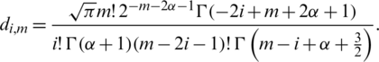
Lemma 3.1. The explicit power form of the normalized Jacobi polynomials , , is given by

where

and

where [z] represents the largest integer less than or equal to z.

Proof. We proceed by induction on n. Assume that relation (10) is valid for (n −1) and (n −2), and we have to prove the validity of (10) itself. Starting with the recurrence relation (3), (for the case ) in the form

where

then, the application of the induction hypothesis twice yields

Eq. (14) may be written in the form

where

and

It is not difficult to see that

where an, k, bn, k are given by (11) and (12), respectively. Therefore

and

and this completes the proof of formula (10).

Lemma 3.2. For all , the following inversion formula holds

where

and

Proof. We proceed by induction on m. Form = 1, the left-hand side equals the right-hand side. Assume that relation (15) is valid, and we have to show that

Multiplying both sides of relation (15) by x, then with the aid of relation (3), (for the case ), and after some rather manipulation, Eq. (16) can be proved.

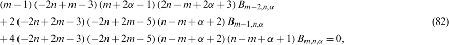
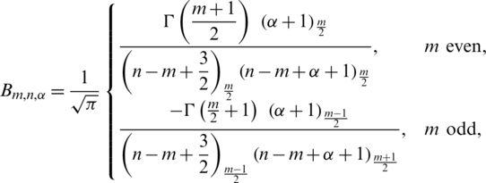
Lemma 3.3. For every nonnegative integer m, we have

Proof. If we set

then, with the aid of Zeilberger’s algorithm [39], Sn, q, m satisfies the following first-order recurrence relation:

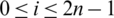
with the initial value

The exact solution for this recurrence relation is

This proves Lemma 3.3.

Now, we are in a position to state and prove the desired derivatives formula.

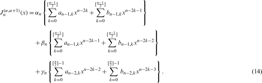
Theorem 3.1. The derivatives of the normalized shifted Jacobi polynomials of any degree and for any order in terms of are given explicitly by

where

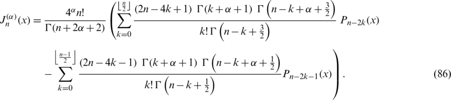
and

Proof. We prove the theorem for , that is, we prove the following formula:

where

and

If we differentiate Eq. (10) q-times with respect to x, and noting the identity

then, we get

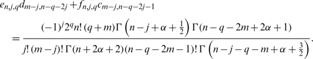
where

Making use of relation (15), enables one to write

where

and

Expanding and and collecting similar terms, then after some rather manipulation, we get

where

and

Now, it is not difficult to show that

and

Finally, making use of Lemma 3.3, An, m, q and Bn, m, q take the forms

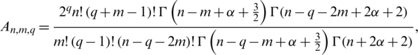
and

Replacing x in (22) by , formula (19) can be obtained. This completes the proof of Theorem 3.1.

Remark 3.1. It is to be noted here that relation (19) may be written in the alternative form

where

Remark 3.2. As a direct consequence of relation (30), the qth derivative of can be easily deduced. This result is given in the following theorem.

Theorem 3.2. The derivatives of the normalized Jacobi polynomials of any degree and for any order in terms of are given explicitly by

where and are given as:

and and are given, respectively, in (20) and (21), or alternatively in the form

where

and is given by (31).

As two direct consequences of Theorems 3.1 and 3.2, the formulas for the high-order derivatives of Chebyshev polynomials of third- and fourth-kinds in terms of their corresponding Chebyshev polynomials can be deduced. These results are given in the following two corollaries.

Corollary 3.1. The derivatives of Chebyshev polynomials of third-kind Vn(x) on [ −1, 1] of any degree and for any order in terms of their original polynomials are given by the following explicit formula:

Corollary 3.2. The derivatives of Chebyshev polynomials of fourth-kind Wn(x) on [ −1, 1] of any degree and for any order in terms of their original formulas are given by

Remark 3.3. The results of Corollaries 3.1 and 3.2 are in complete agreement with those obtained in [6].

Remark 3.4. From now on, we will employ only the polynomials and their shifted ones which will be denoted, respectively, by and . All corresponding results using the polynomials and their shifted ones can be obtained similarly.

4  The Solution of High Even-Order Differential Equations Using

This section is confined to analyzing in detail a spectral Galerkin algorithm for treating numerically even-order BVPs. We will employ the shifted Jacobi polynomials .

Now, consider the following even-order BVPs:

governed by the boundary conditions:

where , and are constant coefficients and is defined as

The philosophy of applying the Galerkin method to solve (36)–(37) is based on choosing basis functions satisfying the boundary conditions (37), and after that, enforcing the residual of Eq. (36) to be orthogonal to these functions. Now, if we set

then, to apply the shifted Jacobi–Galerkin method for solving (36)–(37), we have to find such that

where 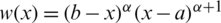, and 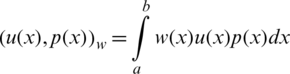is the scalar inner product in the weighted space L2w(a, b).

4.1 The Choice of Basis Functions

In this section, we describe how to choose suitable basis functions satisfying the boundary conditions (37) to be able to apply the Galerkin method to (36)–(37). The idea for choosing compact combinations satisfying the underlying boundary conditions was first introduced in [40,41]. In these two papers, the author selected suitable basis functions satisfying the standard second- and fourth-order BVPs which are considered as special cases of (36). The basis functions were expressed in terms of Chebyshev polynomials of the first-kind and Legendre polynomials. The authors in [42] generalized the proposed algorithms in [40,41]. They suggested compact combinations of ultraspherical polynomials that generalize the Chebyshev of the first-kind and Legendre combinations to solve the even-order BVPs in one- and two-dimensions. The authors in [43] solved the same types of BVPs but by using certain kinds of non-symmetric Jacobi polynomials which are called Chebyshev polynomials of the third- and fourth-kinds. In this section, we are going to generalize the basis functions that derived in [43].

First, consider the case , and set

where the coefficients are chosen such that every member of verifies the following homogeneous boundary conditions:

It is not difficult to see that the boundary conditions (40) along with (39) after making use of identities (5) and (6), (for the case ), lead to the following system of equations in the unknowns :

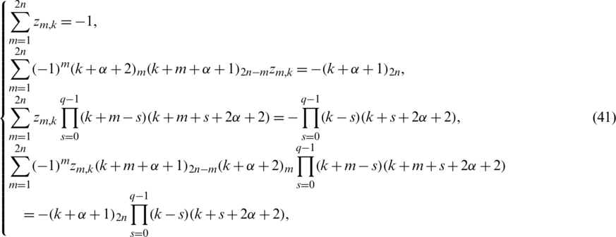
where and

The determinant of the above system is different from zero, hence can be uniquely determined to give

and hence the basis functions 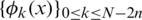take the form:

Remark 4.1. If x in (39) is replaced by , then it is easy to see that the basis functions take the form

and from (43), we see that they have the following explicit expression

satisfies the following boundary conditions

Remark 4.2. If we choose the basis functions in terms of the general parameters normalized Jacobi polynomials , that is

then, the resulting linear system to be solved to find the coefficients Hm, k can not be found in simple forms free of hypergeometric forms except for special choices of their parameters. The choice in this paper enables one to get the simple form of the basis functions in (43).

Now, the basis functions are linearly independent, and hence we have

Now, denote

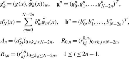
Then Eq. (38) can be transformed into the following matrix system

and the entries of the matrices An and Ri, n, , are given explicitly in the following theorem.

Theorem 4.1. Let the family of basis functions be as taken in (44). Setting , , , . Then

and the nonzero elements of the matrices and R0, n are given explicitly by:

where

and , and zm, k are defined in (31), (9) and (42), respectively.

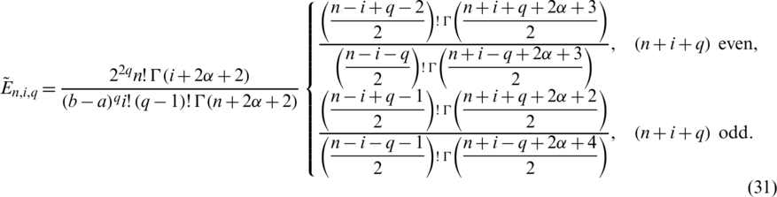
Proof. The nonzero elements of the matrices An, can be obtained with the aid of the derivatives formula (19). Substituting q = 2n in relation (30), yields

where is defined in (31). In virtue of the orthogonality relation (8), one can show for , that

and, accordingly, relation (44) enables one to express the elements ank, j in the form

In particular, it is easy to see that the diagonal elements of An can be simplified to give

Regrading the elements of the matrices Ri, n, , we have

Using relation (30) and the orthogonality relation (8), ri, nkj can be computed to give formulas (50)–(52). Finally, regarding the elements of the matrix R0, n, we have

using the orthogonality relation (8), it can be shown that, for j = k + p, ,

This ends the proof of Theorem 4.1.

The special case corresponding to the choice: , , is of interest. In such case, the system in (47) reduces to a linear system with nonsingular upper triangular matrix for all values of n. The following corollary exhibits this result.

Corollary 4.1. For the case corresponds to , , the system in (47) reduces to , where An is an upper triangular matrix, and its solution can be given explicitly as

where ankk and ankj are given, respectively, by (48) and (49).

Remark 4.3. The following even-order BVP

governed by the nonhomogeneous boundary conditions:

can be transformed to a modified one governed by homogeneous boundary conditions (see [43]).

5  A Collocation Algorithm for Treating Nonlinear BVPs

In this section, we implement and present a numerical algorithm based on a collocation method to solve even-order nonlinear BVPs. The basic idea is based on employing the operational matrix of derivatives of the shifted Jacobi polynomials . First, the following corollary is essential in the sequel.

Corollary 5.1. The first derivative of the polynomials can be written explicitly as

where

Proof. Direct from Eq. (30), setting q = 1.

Now, if we define the following vector

then, it is easy to see that

where M is the operational matrix of derivatives whose entries are defined as:

Now, consider the following nonlinear even-order BVPs:

subject to the first-kind of boundary conditions:

or the second-kind of boundary conditions:

Now, consider an approximate solution of the form

This approximate solution can be expressed as

where

and is defined in (63).

In virtue of Eq. (64), it is easy to express the th-derivative of uN(x). In fact, we can write

Based on relation (71), the residual of Eq. (65) can be written as

Now, for the sake of obtaining a numerical solution of (65), a collocation method is applied. More precisely, the residual in (72) is enforced to vanish at suitable collocation points. We choose them to be the distinct zeros of the polynomial , that is we have

Furthermore, the boundary conditions (66) yield the following (2n) equations:

while, the boundary conditions (67) yield the following (2n) equations:

Merging the (N + 1) equations in (73)–(75), or the (N + 1) equations in (73), (76) and (77), we get a nonlinear system in the expansion coefficients ak which can be solved with the aid of Newton’s iterative method. Thus an approximate solution uN(x) can be found.

6  Connection Formula between the Polynomials and the Shifted Legendre Polynomials

This section is confined to present the connection formula between the polynomials and the shifted Legendre polynomials on [a, b]. This connection formula will be of important interest in investigating the convergence and error analysis in the subsequent section. To this end, the following theorem which links between two different parameters Jacobi polynomials is needed.

Theorem 6.1. For every nonnegative integer n, the following connection formula holds:

Proof. The connection formula between two different parameters classical Jacobi polynomials is given by [44]

with

Taking into consideration relation (2), the connection formula (78) can be obtained.

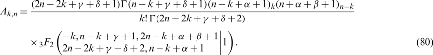
Lemma 6.1. Let m and n be two nonnegative integers. The following reduction formula holds

Proof. If we set

then, with the aid of Zeilberger’s algorithm, it can be shown that the following second-order recurrence relation is satisfied by

with the initial values

The recurrence relation (82) can be solved exactly to give

and, therefore, the reduction formula (81) can be followed.

Now, we are going to state and prove an important theorem that concerns the connection formula between and the shifted Legendre polynomials P*k(x).

Theorem 6.2. The connection formula between the shifted normalized Jacobi polynomials and the shifted Legendre polynomials P*k(x) can be written explicitly in the form

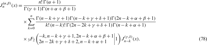
where the connection coefficients are given by

Proof. To prove the connection formula (83) with coefficients in (84), we prove first the formula on [ −1, 1], that is, we prove the formula

The last relation can be written alternatively in the form

Setting and in Eq. (78) yields the following formula

If we make use of Lemma 6.1, then the last formula, after some computations can be transformed into the form in (86), and therefore, relation (85) is proved. Replacing x by in (85) gives (83). Theorem 6.2 is proved.

7  Study of the Convergence and Error Analysis

In this section, we state and prove some results concerning the convergence analysis of the proposed expansions in Sections 4 and 5. First, we mention some theoretical prerequisites. The following lemmas and theorems are needed. Let us agree on the following notation: For two positive sequences ai, bi, we say that if there exists a generic constant c such that .

7.1 Prerequisites

Lemma 7.1. Reference [45] Let Iqk(x) denote the q-times repeated integrals of shifted Legendre polynomials, that is

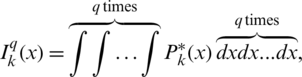
then, Iqk(x) can be expressed in terms of shifted Legendre polynomials by the formula

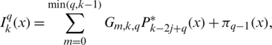
where is a polynomial of degree at most (q −1), and the coefficients Gm, k, q are given explicitly by

Lemma 7.2. Let Iqk(x) be defined as in the above lemma. The following estimate holds

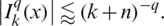
Proof. The lemma can be proved with the aid of the repeated integrals formula in Lemma 7.1 and noting the well-known inequality: .

Lemma 7.3. The connection coefficients in the connection problem (83), which expressed explicitly in (84) satisfy the following estimate

Proof. The result can be easily followed from the explicit formula of the connection coefficients in (84).

Lemma 7.4. For all , the following estimate is valid

Proof. From the connection formula (83), and noting that , we get

We will prove (89). We consider the proof if n is even. The case if n is odd can be treated similarly. From (90), we can write

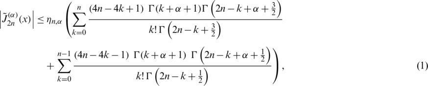
with

With the aid of Zeilberger’s algorithm, it is not difficult to show that

and

and accordingly, we get

The proof is now complete.

7.2 Convergence Analysis

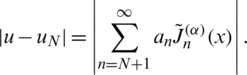
Now, we are ready to state and prove some lemmas and theorems concerning the convergence of the truncated approximate solutions and the estimate for the truncation error of the proposed expansions in Sections 4 and 5. We first prove our results for the proposed expansion in Section 5. Assume that the exact and approximate expansions are respectively as follows:

and

From now on, and for more convenience, let us agree on the following notations:

Theorem 7.1. If the exact solution in (92) is Cq-function, for some q > 3, and for , then the following statements are correct:

  1.  The expansion coefficients an satisfy the following estimate:

  2.  The series in (92) converges uniformly.

Proof. Due to (8), the expansion coefficients an are given by

It is clear from relation (9) that , and consequently

Thanks to the connection formula (83) that links with the shifted Legendre polynomials, we have

and in virtue of Lemma 7.3, the last inequality gives

Now, if we apply integration by parts q-times and along with the following result obtained by Leibniz’s Theorem

the following estimate can be obtained

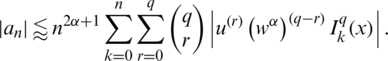
Now, the direct application of Lemma 7.2, and after performing some manipulations, yield

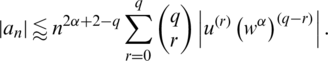
By the hypothesis of the theorem, precisely, the boundedness of the derivatives u(r), we get

which completes the proof of the first-part of the theorem.

For the second part, we have

and with the aid of the first result of this theorem along with Lemma 7.4, we get

Taking into consideration the condition: , and applying the integral test, the desired series converges uniformly, and this completes the proof of the second-part of the theorem.

Theorem 7.2. Under the hypotheses of Theorem 7.1, the following truncation error estimate is valid:

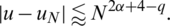
Proof. Using relations (92) and (93), it is clear that

Now, by the result of Theorem 7.1 along with Lemma 7.4 yield the following inequality:

Now, based on the asymptotic behaviour of the Riemann–Hurwitz function, we have

which completes the proof of the theorem.

Remark 7.1. The main idea to investigate the convergence and error analysis of the expansion that used in Section 4 is built on transforming the basis functions (45) into another suitable form, and after that perform similar procedures to those followed in Subsections 7.1 and 7.2. More precisely, the following theorem is the key for such study. It can be proved through induction.

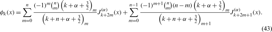
Theorem 7.3. Let be the basis functions in (45). The following identity holds for every positive integer n

8  Numerical Results

In this section, we give some numerical results obtained by using our two proposed algorithms, namely, shifted Jacobi Galerkin method (SJGM) and the shifted Jacobi collocation method (SJCM) which presented, respectively, in Sections 4 and 5. Furthermore, some comparisons between our two proposed algorithms with some other methods exist in the literature are presented hoping to show the efficiency and accuracy of our proposed methods. In this section, the symbol N refers to the number of retained modes. In addition, u(x) is the exact solution and uN(x) is the corresponding approximate solution and the error is denoted by E where .

Example 1. Consider the sixth-order linear boundary value problem [46,47]

subject to the boundary conditions

The exact solution for this problem is: .

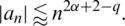
Tab. 1 lists the maximum absolute errors E for various choices of N, c, and . In Tabs. 2 and 3, comparisons between our proposed SJGM and the two methods developed in [46,47] are displayed. In addition, in Fig. 1, we depict the Log-error plot of Example 1 for the case corresponds to various values of N and .

Table 1: Maximum absolute error of E for Example 1

Table 2: Errors at xi for N = 12 and c = 10 for Example 1

Table 3: Errors at xi for N = 12 and c = 1000 for Example 1

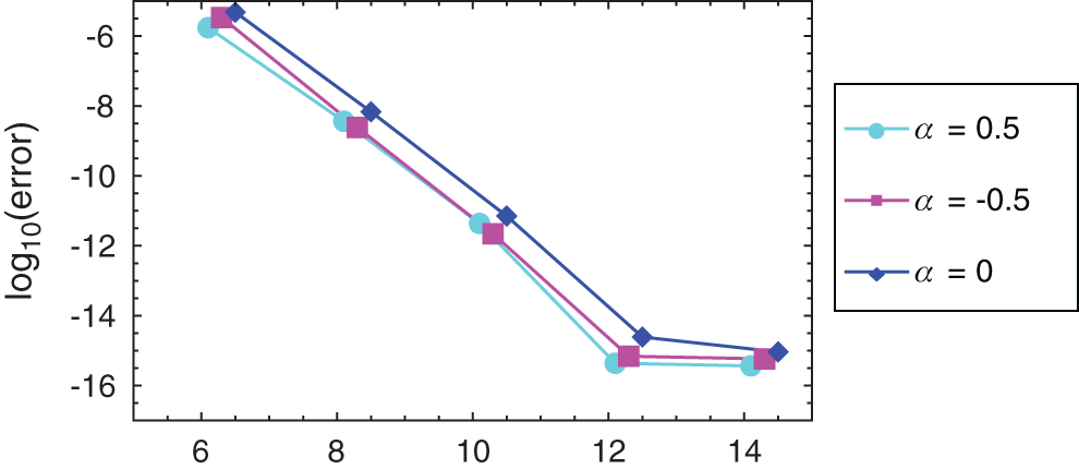
Figure 1: Log-error of Example 1 for c = 1

Remark 8.1. The results in Tab. 1 show that the case corresponding to third-kind Chebyshev polynomials does not always give the best results.

Example 2. Consider the eighth-order linear boundary value problem [48]

subject to the boundary conditions

The exact solution for this problem is: u(x) = (1 − x)ex.

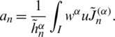
Tab. 4 presents the maximum absolute error E for some choices of and N, while Tab. 5 lists a comparison between our proposed algorithm with the absolute errors obtained by the method proposed in [48]. In Fig. 2, we depict the absolute error plot of Example 2 for the case corresponds to N = 14 and various values .

Table 4: Maximum absolute error of E for Example 2

Table 5: Errors at xi for N = 14 for Example 2

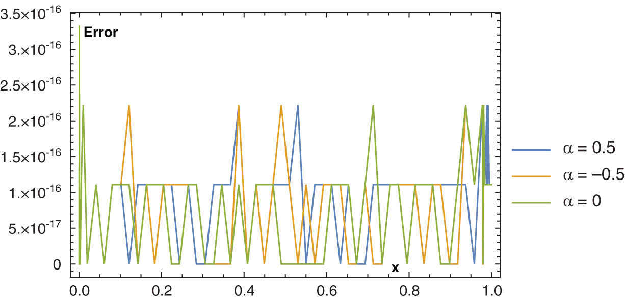
Figure 2: Absolute error plot of Example 2

Example 3. Consider the eighth-order nonlinear boundary value problem [49,50]

subject to the boundary conditions

The exact solution for this problem is: .

Tab. 6 lists the maximum absolute error E for various values of N and . For the sake of comparison with other methods, we compare the best errors obtained from the application of our algorithm with those obtained by the two methods developed in [49,50]. Tab. 7 displays these results.

Example 4. Consider the twelfth-order nonlinear boundary value problem [51,52]

subject to the boundary conditions:

The exact solution for this problem is: u(x) = 2 ex.

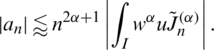
Tab. 8 presents the maximum absolute error E for some choices of and N, while Tab. 9 lists a comparison between our proposed algorithm for N = 21 for various values of with the best errors obtained by the methods developed in [51,52]. In Fig. 3, we depict the absolute error plot of Example 4 for the case corresponds to N = 21 and various values .

Table 6: Maximum absolute error of E for Example 3

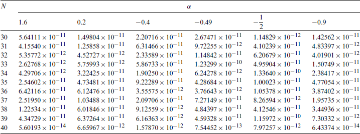
Table 7: Best errors for N = 40 for Example 3

Table 8: Maximum absolute error of E for Example 4

Table 9: Best errors for Example 4

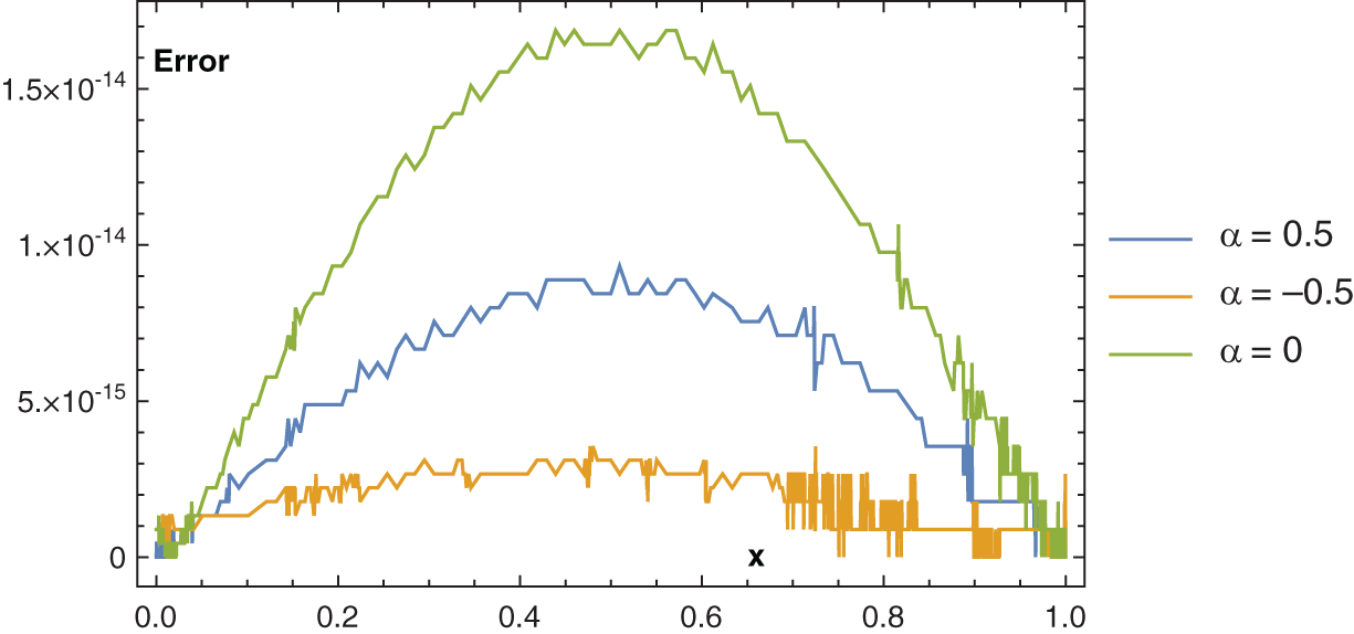
Figure 3: Absolute error plot of Example 4

9  Conclusions

Some direct algorithms for treating both linear and nonlinear BVPs were analyzed and presented. The proposed solutions are spectral. Two different approaches were presented for solving such problems. In the linear case, a Galerkin approach is followed. The basis functions are expressed in terms of certain Jacobi polynomials which generalize the well-known Chebyshev polynomials of the third- and fourth-kinds. Another collocation approach is followed for the treatment of both linear and nonlinear BVPs. A new operational matrix of derivatives of certain shifted Jacobi polynomials was constructed for this purpose. The presented numerical results show that the expansion of the third-kind of Chebyshev is not always the best in approximation. Moreover, the numerical results show that our algorithms are applicable and of high accuracy.

Acknowledgement: The authors would like to thank the anonymous reviewers for carefully reading the article and also for their constructive and valuable comments which have improved the paper in its present form.

Funding Statement: The authors received no specific funding for this study.

Conflicts of Interest: The authors declare that they have no conflicts of interest to report regarding the present study.

This work is licensed under a Creative Commons Attribution 4.0 International License, which permits unrestricted use, distribution, and reproduction in any medium, provided the original work is properly cited.