Computer Modeling in Engineering & Sciences

DOI: 10.32604/cmes.2021.014493

ARTICLE

Geometric Multigrid Method for Isogeometric Analysis

Houlin Yang1, Bingquan Zuo1,2,*, Zhipeng Wei1,2, Huixin Luo1,2 and Jianguo Fei1,2

1Key Laboratory of Metallurgical Equipment and Control Technology Ministry of Education, Wuhan University of Science and Technology, Wuhan, 430081, China
2Hubei Key Laboratory of Mechanical Transmission and Manufacturing Engineering, Wuhan University of Science and Technology, Wuhan, 430081, China
*Corresponding Author: Bingquan Zuo. Email: zuobingquan@gmail.com
Received: 02 October 2020; Accepted: 10 December 2020

1  Introduction

In recent years, as a numerical method for solving partial differential equations (PDEs), isogeometric analysis [1] (IGA) has been widely concerned and studied. The basic idea of IGA: Based on the isoparametric element theory, geometric splines can not only describe the exact geometric modeling but also the solution space of numerical methods, which can unify the geometric model and the analytical model. Therefore, the spline information in CAD model is directly used as the initial mesh in IGA. Since it was proposed, most of the research on IGA has focused on parametric modeling and physical spatial discretization. However, when dealing with large-scale problems, it is still a problem to solve the system of linear equations which are obtained from the geometric discretization. The reason is that the direct solution is inefficient and usually requires targeted development of faster and more efficient iterative solver.

The multigrid method [2,3] (MG) is often used as an efficient iterative algorithm to solve large-scale linear equations. The main idea is to eliminate high-frequency errors through fine mesh smoothing, coarse grid correction to eliminate low frequency errors, and an iterative strategy for fine grid and coarse grid cycles. According to the different mapping matrix generation methods, the MG can be divided into two types: geometric multigrid method (GMG) and algebraic multigrid method (AMG). Usually the AMG is more widely used then the other because it obtains different level meshes in an algebraic way instead of constructing them, which may be complicated in some cases [4]. However, the IGA directly generates the hierarchical mesh through the refinement method (p-refinement, h-refinement, k-refinement), which encourages us to implement the GMG in IGA.

It seems natural to extend these methods to IGA, and several remarkable works has been made in recent years. MG for IGA based on classical concepts have been considered in [5,6], and a classical multilevel method in [7]. An approach to local refinement in IGA based on a full multigrid method(FMG) can be found in [8]. The related studies mainly include Gahalaut et al. [9] applied multigrid to IGA, and did not propose the concept of mapping matrix; Hofreither et al. [10] proposed a robust error approximation. These studies above mainly focus on the implement of MG in IGA. And the efficiency in the adaptation process has been studied. Other research mainly includes Guo [11] to improve efficiency through parallel computing and multi-grid method, Liu et al. [12] combined conjugate gradient method with multi-grid method, and Chen et al. [13] based on geometric analysis such as least squares coupling multigrid method. Recently, in [14] some progress has been made by using a Richardson method preconditioned with the mass matrix as a smoother (mass-Richardson smoother). Similar techniques have been used to construct symbol-based multigrid methods for IGA, see [15,16]. However, all the above research uses the coordinate mapping relationship in the process of geometric mesh construction to modify the traditional algebraic multigrid iterative process but ignore the stiffness information discretely obtained during isogeometric subdivision. In addition, the extension matrix transposition is directly used in the construction of restriction matrix, which will lead to the confusion and imbalance of mapping relationship.

Based on previous generations, this paper uses the geometric information discretized by isogeometric subdivision to couple the MG with IGA and its application. Especially for the numerical algorithms such as IGA, we use geometric method to optimize them in the shortcomings of AMG, and it has integrated into the process of FMG.

2  Isogeometric Analysis

2.1 B-Splines and NURBS Basis Functions

Like FEM, IGA also have shape functions, not the Lagrange interpolation functions but the spline basis functions. As the two common spline functions used in CAD, B-spline and NURBS are briefly introduced below. With a given node vector, the B-spline basis function [17] can be recursively defined as:

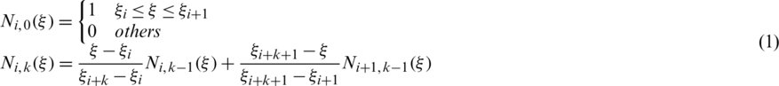
where the one-dimensional knot vector is a set of non-decreasing sequences between 0 and 1. k is the degree of the basis function (p = k + 1 is the order of the basis function). n is the number of basic functions, which is numerically equal to the number of control points.

If the basis function of B-spline is multiplied by an appropriate weight w, the non-uniform rational B-spline (NURBS) can be introduced. Its expression is:

2.2 The Framework of Multigrid Isogeometric Analysis

FEA and IGA have the same theoretical basis (i.e., the weak form of partial differential equation). Take the common elliptic partial differential equation as an example:

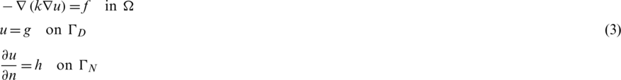
where is the open and bounded Lipschitz domain and the boundary is , , ; Given source term ; Symmetric positive definite matrix ; Dirichlet boundary value 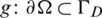; Neumann boundary value .

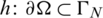It is assumed that the physical domain is represented by a parameter domain mapping , . Using the control point cij, F can be defined by NURBS as:

The weak form of the differential equation is obtained by multiplying with the trial function and integrating in the domain . Let and , then the equation becomes . According to Green’s method, the linear equations are obtained by discrete assembly:

The detailed process can be seen in [18,19].

2.3 Isogeometric Subdivision

Based on the requirements of light weight, modern CAD systems follow the principle of sufficient enough when characterizing models [20]. So, the spline order in CAD is low usually, just meeting the basic characterization needs, and the node of the parameter domain is relatively sparse. But the order of the shape function (spline basis function) and the grid size (knot vector interpolation space scale) have a great impact on the analysis accuracy. As a result, the first step in IGA is subdivision, which works like the refinement in FEM, but with a different method. Therefore, it is necessary to introduce the subdivision process before constructing the isogeometric multiple meshes.

There are mainly three subdivision methods [21] in IGA, they are p-refinement, h-refinement and k-refinement. All these subdivision methods can keep the original shape the same. The changes are mainly at the spline order and knot vector. In particular, the p-refinement retains the original parameter domain grid and only increases the order of the basis function; the h-refinement does not change the basis function order but reduces the grid size to construct a finer parameter domain grid. As a combination of p-refinement and h-refinement, k-refinement increase the order of basis function firstly, and then refines the knot vector.

Taken the one-dimensional h-refinement as an example for introduction. Inserting the knot into the knot vector at one time can get the new knot vector , then the corresponding coordinate calculation formula of the new spline control point can be obtained [22]:

where is the coordinate of the original spline control point.

If k = 3 (the cubic B-spline), Formula (6) can be written as follow:

where, the coefficients can be calculated as follows:

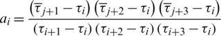
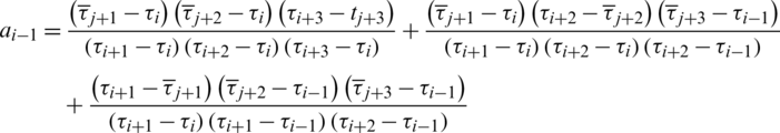
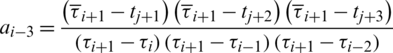
During p-refinement process, the degree of the spline curve is raised once, and the shape and continuity of the curve remain unchanged. Cohen [23] offered a solution to calculate the new control points:

where recursively as follows:

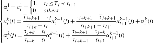
K-refinement is a combination of h-refinement and p-refinement. In order to ensure the continuity of elements, k-refinement is often defined as “first upgrade, then insert nodes” in IGA. This means, for the B-spline curve of order p, the order is elevated to q by p-refinement firstly, and then knots inserting is taken by h-refinement.

3  Multigrid Method

For FEM, most of MG method uses the algebraic multigrid method to construct interpolation operator and coarse the initial grid to get different hierarchical grid. In IGA, the geometric model is constructed from coarse to fine. There are different levels of grid naturally, and the mapping matrix between each level can be obtained from the subdivision process. In addition, each level has its own stiffness matrix and righthand vector. If this advantage is used to combine the multigrid method with IGA, the efficiency of solution would be improved.

3.1 Multigrid Mapping Matrix

3.1.1 Classical Algebraic Multigrid Mapping Matrix

In AMG, the main work is focused on constructing the interpolation matrix by coarsen the fine mesh, coarsening refined net to get rough grid . And the coarse grid is a subset of the fine grid defined with Cm, using Fm to define the remaining set , when , , the point i is strongly connected to point j. Let define all the strong connection points of point i, then the strong connection rough set is and the interpolation matrix refers to the interpolation formula given by Chang et al. [24].

For MG, the mapping matrix is important. And its generation can affect the computational efficiency of MG directly. So, it is necessary to compare the generation rate of mapping matrix under different degrees of freedom. the time-consuming of mapping matrix generation (using Chang’s method) in Tab. 1 shows that the time of generating the mapping matrix of the algebra multigrid rises sharply with the increase of degrees of freedom. Obviously, a faster constructing method for mapping matrix will be helpful for the implement of MG.

Table 1: The generation rate of mapping matrix

3.1.2 Suitable for Isogeometric Analysis of Multigrid Mapping Matrix

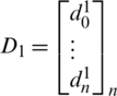
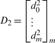
As discussed in Chapter 2.3, in the subdivision of IGA can generate the mapping relationship between new and old control points Dm and Dn. It is assumed that the relationship between (on fine grid) and (coarse grid) also satisfies this relationship. According to the formula (7), the extension matrix from coarse to fine corresponding to h-refinement can be expressed as:

in the formula,

The corresponding linear relation is that the non-zero element in row vector r is numbered as the old control point number related to the new control point, which is usually a continuous interval segment.

P-refinement extended matrix can be obtained according to the calculation of Formula (8):

Therefore, the extended matrix of k-refinement is:

In theory, the restriction matrix from fine grid to coarse grid is the generalized inverse matrix of extension matrix , but it is difficult to calculate the inverse matrix of extension matrix , and there are stability problems and limitations in inversion calculation. Therefore, in this paper, transposed matrix is chosen as generalized inverse, P = RT. But in fact, the mapping matrix obtained by transpose cannot accurately represent the mapping relationship from coarse grid to fine grid, so the mapping matrix is modified by parameter here:

in the formula, , , .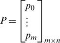

Since the control point D is a coordinate vector, the difference between the positive and negative coordinates will affect the effect of the correction. To ensure the positive correction of the parameter , the analysis model can be translated to the first quadrant to ensure that the control point coordinates are greater than zero.

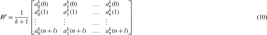
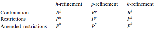
In IGA, the mapping matrix obtained by different refinement strategies are shown in Tab. 2. The detailed process can be referred to [25].

Table 2: Mapping matrix

Based on one-dimensional subdivision, two-dimensional subdivision only needs to subdivide in directions at the same time to get mapping matrix and , and then get the mapping matrix by global numbering of coarse and fine meshes. is the number of control points of the grid. can be represented by Eq. (13).

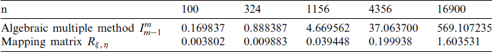
A time-consuming compare of mapping matrix generation between this method and AMG is given in Tab. 3. With the freedom increase, more time can be saved in pre-processing stage of MG.

Table 3: The generation rate of mapping matrix

3.2 Multigrid Algorithm

3.2.1 Geometric Modification of Algebraic Multigrid Method

The multigrid method is divided into initial period and calculation stage. In the initial period, GMG is based on the subdivision of the solution domain to get the grid of different scales. AMG only uses the information of coefficient matrix in algebraic equations to construct multigrid, and the method is consistent in the iterative solution stage. In order to improve the implement of AMG in IGA, geometric information will be introduced to AMG, what is called Geometric modification of algebraic multigrid method (GMG).

1. Initial period

  1.  The nested grid layer 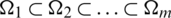is constructed by subdivision, and the extension matrix from layer m −1 grid to layer m is stored. The mapping matrix from layer m grid to layer m −1 is modified according to Eq. (12).

  2.  Multigrid 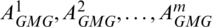is obtained by discretizing PDEs with the method of IGA, so the Right items .

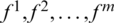2. Calculation stage

The iterative process of multigrid method (GMG) is given above. For a given parameter space , a rough gird for IGA can be built. Though refinement, multilevel grids can be constructed., so the limit matrix of layer m to layer m −1 and the extension matrix from m −1 to m . Parameter d in GAMG determines how to access each layer, as shown in Fig. 1, d = 1 is a V-type cycle and d = 2D is a W-type cycle. The traditional AMG, the left term of the coarse grid is calculated using the mapping method, . In GMG, the corresponding Am of each geometric level can be calculated directly. That means, GMG in this paper introduces geometric information as a more selection of residual and selects the smaller residual as the next relaxation iteration by comparing the residual between geometric grid and algebra grid.

Figure 1: Multi-grid cycle

As for the iteration of relaxation operator , v1 = v2 = 2 represents the number of times of relaxation. In order to get the iteration structure, Am is divided into Am = Mm − Nm, and its iterative format can be written as:

Mm is selected to obtain various iterative methods for relaxation. Jacobi, Gauss–Seidel and SOR iterations are commonly used. For rough grid correction, both the residual and error satisfy the residual equation Amem = rm, so em −1 can be solved by the same relaxation operator S.

3.2.2 Full Multigrid Method

As known to all, Am and fm are discretized on each level grid in IGA, in order to make full use of these information, a full multigrid method (FMG) method suitable for IGA is established.

In the loop process of FMG, both AMG and GMG can be selected as solving algorithm on each layer, hence the accuracy of each layer can be guaranteed. Besides, and with the help of the extension matrix , the results can be interpolation to the previous layer as the initial solution which can be useful to reduce the iteration steps. As shown in Fig. 2, the FMG process is as follows:

Figure 2: Full multigrid method

4  Numerical Examples

In order to verify the validity of the algorithm, this paper has carried out the verification on the Poisson equation and Reynolds equation.

According to the relationship between residual norm and error norm: , the convergence of the residual and the error is consistent.

The relative error can be expressed as follows:

The convergence rate is defined as:

The algorithm is written in OCTAVE, the computer processor is Core i5-4570, with 3.20 GHz frequency. We contrast the convergence and calculation time of different subdivision strategies. The unified cycle format is V cycle, the number of grid layers m = 3, and the subdivision mode of coarse grid to fine grid is , corresponding to the 6-bit coding (such as 102026) shown in the figure below, respectively. Select the corresponding subdivision strategy from Tab. 5 (Reynolds) and Tab. 8 (Poisson), and the relaxation algorithm selects Gauss–Seidel iteration, and the number of internal iterations is controlled to be v1 = v2 = 2.

4.1 Reynolds Equation Model

The piston-cylinder liner is used as a lubrication system, and the oil film pressure is derived based on the Reynolds equation. Fig. 3a shows the piston liner system, and the area of lubricating film is shown in Fig. 3b. Based on the Navier–Stokes equations and the mass continuity equation, the Reynolds equation [26,27] can be established as follows:

where is the lubricant density, p is the oil film pressure, is the dynamic viscosity, u0 and uh are the oil film circumferential speeds on the piston and the cylinder liner surface, v0 and vh are the film shaft speed on the piston and the cylinder liner surface, h is the film thickness, t is time.

Figure 3: Piston-cylinder liner lubrication system (a) piston-cylinder system (b) oil film lubrication area

Since the lubrication area is symmetrical relative to the plane , only the right half needs to be considered. In general, the piston moves periodically, and the values of density and viscosity will change with the change of load value. However, in order to simplify the numerical model, the values of density and viscosity are taken as constant. The calculation parameters of oil film pressure are shown in Tab. 4.

Table 4: Calculate parameters

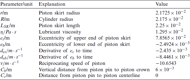
Table 5: Number of control points from MG based on different refinement strategies

The motion parameters of the piston-cylinder liner model have been given above, and the relevant detailed derivation process is referred to [28,29].

When the Reynolds equation is discretized, the knot vector of the initial parameter domain is v = u = [0 0 1 1]. In the initial state, given different p, h, k-refinement strategies will get different levels of grid control points.

In the case of h-refinement, n is the thinnest grid, and the appropriate coarse grid is selected to make it have the fastest convergence rate. It can be seen from Tab. 6 that when k is constant, the grid size is independent of the convergence rate. Since the Reynolds equation is an elliptic equation of second order, so it has the fastest convergence rate at k = 2. When k increases, the convergence rate decreases sharply.

Table 6: Convergence rate

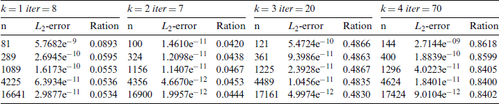
Fig. 4 only shows the comparison between h-refinement and k-refinement in order to explore the influence of different refinement strategies on the convergence rate. The broken lines in the figure indicate the number of subdivisions of each layer of the grid. For example, 252627 represents the second-order fifth-level grids, the second-order sixth-level grids and the second-order seventh-level grids. The figure below is similar. The traditional AMG and GMG are used to compare the convergence of different degrees of freedom and spline degree k. The convergence rate of AMG and GMG iterations are shown in Fig. 5. Tab. 7 shows the CPU calculation time of the AMG algorithm and the GMG algorithm. It can be seen that: when the number k is constant, the convergence rate of AMG and GMG is almost the same under different grid sizes. Due to the different ways in which the coarse grid matrix is generated, the non-zero elements of the matrix A are different. As shown in Fig. 6, nz is the number of non-zero elements. The band length in the GMG matrix A is reduced globally and locally, and the number of non-zero elements is less than that in the AMG matrix. Therefore, when the degree of freedom is large, the GMG of the natural discrete matrix A can save more time and computing resources. Meanwhile, as the right items of different levels of are also produced in the discrete process, FMG can be used to calculate the original right items in the current layer. It can be seen from Fig. 7 that the full multiple cycles have superior initial values in the iterative calculation process, and the desired error accuracy can be obtained in less iterations.

Figure 4: Relative error of refinement strategy (a) H-refinement relative error (b) K-refinement relative error

Figure 5: Relative error between AMG and GMG (a) k = 1 (b) k = 2 (c) k = 3 (d) k = 4

Table 7: CPU calculation time of AMG and GMG

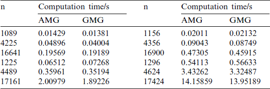
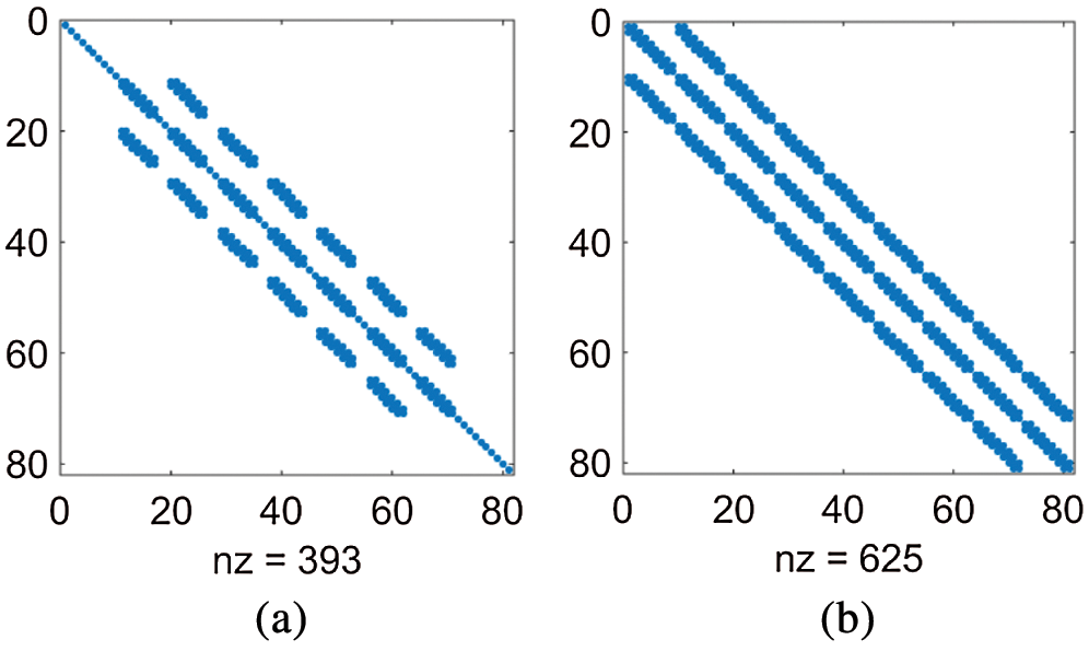
Figure 6: Coarse grid matrix A (a) GMG (b) AMG

Figure 7: Relative error between FMG and GMG

4.2 Poisson Equation Model

The equation of the two-dimensional Poisson problem with Dirichlet boundary conditions in the domain with the following expression:

The domain is the quarter-ring of the inner radius Ri = 1 and the outer radius Re = 2 is shown in Fig. 8. When the right term heat source is , the analytical solution is .

Figure 8: Two dimensional poisson heat transfer problem

For the parameter domain knot vector of two-dimensional Poisson equation is v = u = [0 0 0 1 1 1] in the initial state, the convergence and calculation time of subdivision strategy are compared under the working environment mentioned above. The related calculated data correspond to the Reynolds equation are listed below.

Tab. 9 discusses the influence of the choice of grid level on convergence in the AMG algorithm under different subdivision situations. Fig. 9 only shows the comparison between h-refinement and k-refinement in order to explore the influence of different refinement strategies on the convergence rate. It can be seen from the figure that the mapping matrix satisfies the mapping relationship between the control points when there is a large gap between the number of control points of the coarse and fine grid, whether h-refinement or k-refinement. For the assumed scale series between and are large, the linear distortion leads to the inaccurate mapping relationship, and the convergence rate is not converged as expected. Within a certain range of the number gap between the coarse and fine grid points, the convergence rate of h-refinement is different in the early iteration, but the convergence curve tends to coincide in the later 10 iterations, while the trend of k-refinement only convergence rate is the same. Therefore, the selection of the appropriate grid hierarchy is beneficial to the convergence of the multi-grid method. Fig. 10 shows the relative error of the AMG algorithm and the GMG algorithm. Tab. 10 shows the CPU calculation time of the AMG algorithm and the GMG algorithm. Although the convergence rate of the AMG algorithm and the GMG algorithm is almost the same in the verification of the Reynolds equation, the GMG algorithm still saves more time in the initial period calculation.

Table 8: Number of control points from MG based on different subdivision strategies

Table 9: Convergence rate

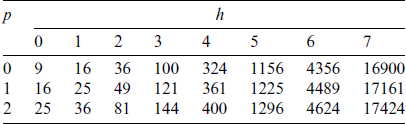
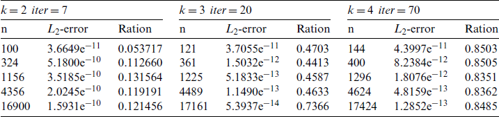
Figure 9: Relative error of refinement strategy (a) H-refinement relative error (b) K-refinement relative error

Figure 10: Relative error between AMG and GMG (a) k = 2 (b) k = 3 (c) k = 4

Table 10: CPU calculation time of AMG and GMG

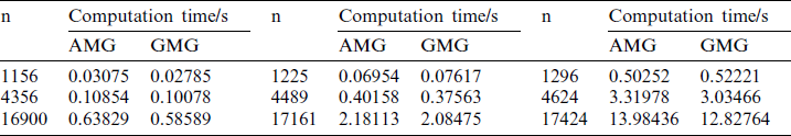
Fig. 11 shows the convergence comparison between FMG and GMG under the Reynolds equation model. It can be seen that: at the start stage, with the help of the good initial value, the FMG algorithm has a better accurate result, but the convergence tends to be consistent with others in the later stage.

Figure 11: Relative error between FMG and GMG

In this paper, the algebraic multigrid method and the geometric analysis of the natural discrete stiffness matrix are used instead of the transpose generation matrix , and the geometric multi-grid method and the algebraic multigrid method are compared. Numerical results show that: convergence rates of the two methods keep consistent, but GMG reduces the time cost at the initial period. For the subdivision strategies of different levels (3 levels), the convergence rate of h-refinement intermediate layer is faster when it is closer to the fine grid, and the convergence rate of k-refinement intermediate layer is faster when it is in the middle of coarse and fine grid. When FMG is applied to IGA, its convergence rate is faster than that of GMG.

5  Conclusion

Based on the framework of IGA, the analytical models of Reynolds equation and Poisson equation are established, and multigrid is applied to the IGA. According to its solving process and method, a calculation program was developed in OCTAVE (FMG based on GMG modified the traditional AMG). The convergence rate of the iteration is independent of the size of the discrete mesh, so the multigrid method has the optimal computational complexity. When the degree of freedom of fine grid is determined, the degree of freedom of coarse grid can be reduced and the boundary information can be quickly spread to the whole, which can not only accelerate the convergence rate but also save the cost of calculation time. However, the selection of grid level also affects the convergence accuracy. In particular, the selection of the middle level has a greater impact on the results, and the performance of the middle grid close to the top grid is better. As for the combination of FMG and IGA, the results show that the algorithm can make full use of IGA to discretize the geometric information of each layer. Compared with the V-cycle, it has a faster initial convergence speed, but it is consistent with conventional algorithms in the later stage. How to make better use of the existing information to accelerate calculation efficiency and improve calculation accuracy is the direction we will continue to study in the future.

Funding Statement: This research was supported by the Natural Science Foundation of Hubei Province (CN) (Grant No. 2019CFB693), the Research Foundation of the Education Department of Hubei Province (CN) (Grant No. B2019003) and the open Foundation of the Key Laboratory of Metallurgical Equipment and Control of Education Ministry (CN) (Grant No. 2015B14). The support is gratefully acknowledged.

Conflicts of Interest: The authors declare that they have no conflicts of interest to report regarding the present study.

References

 1.  Nguyen, V. P., Anitescu, C., Bordas, S. P., Rabczuk, T. (2015). Isogeometric analysis: An overview and computer implementation aspects. Mathematics and Computers in Simulation, 117, 89–116. DOI 10.1016/j.matcom.2015.05.008. [Google Scholar] [CrossRef]

 2.  Briggs, W. L., Henson, V. E., Mccormick, S. F. (2000). A multigrid tutorial. 2nd edition. Philadelphia, PA: Society for Industrial and Applied Mathematics. [Google Scholar]

 3.  Tai, C. H., Zhao, Y. (2003). Parallel unsteady incompressible viscous flow computations using an unstructured multigrid method. Journal of Computational Physics, 1(1), 277–311. DOI 10.1016/j.jcp.2003.07.005. [Google Scholar] [CrossRef]

 4.  Stüben, K. (2001). A review of algebraic multigrid. Journal of Computational and Applied Mathematics, 1–2, 281–309. DOI 10.1016/S0377-0427(00)00516-1. [Google Scholar] [CrossRef]

 5.  Hofreither, C., Zulehner, W. (2015). Spectral analysis of geometric multigrid methods for isogeometric analysis. Numerical Methods and Applications, 8962, 123–129. DOI 10.1007/978-3-319-15585-2_14. [Google Scholar] [CrossRef]

 6.  Hofreither, C., Zulehner, W. (2016). On full multigrid schemes for isogeometric analysis. Domain Decomposition Methods in Science and Engineering, 22, 267–274. DOI 10.1007/978-3-319-18827-0_25. [Google Scholar] [CrossRef]

 7.  Buffa, A., Harbrecht, H., Kunoth, A., Sangalli, G. (2013). BPX-preconditioning for isogeometric analysis. Computer Methods in Applied Mechanics and Engineering, 265, 63–70. DOI 10.1016/j.cma.2013.05.014. [Google Scholar] [CrossRef]

 8.  Chemin, A., Elguedj, T., Gravouil, A. (2015). Isogeometric local h-refinement strategy based on multigrids. Finite Elements in Analysis and Design, 100, 77–90. DOI 10.1016/j.finel.2015.02.007. [Google Scholar] [CrossRef]

 9.  Gahalaut, K. P., Johannes, K., Satyendra, T. (2013). Multigrid methods for isogeometric discretization. Computer Methods in Applied Mechanics And Engineering, 100, 413–425. DOI 10.1016/j.cma.2012.08.015. [Google Scholar] [CrossRef]

10. Hofreither, C., Takacs, S., Zulehner, W. (2017). A robust multigrid method for isogeometric analysis in two dimensions using boundary correction. Computer Methods in Applied Mechanics and Engineering, 316, 22–42. DOI 10.1016/j.cma.2016.04.003. [Google Scholar] [CrossRef]

11. Guo, L. C. (2013). Improving the computational efficiency of isogeometric analysis via parallel computing and multigrid methods. Hefei, China: University of Science and Technology of China. [Google Scholar]

12. Liu, S., Chen, D. X., Feng, Y. X., Xu, Z. L., Zheng, L. K. (2014). A multigrid preconditioned conjugate gradient method for isogeometric analysis. Applied Mathematics & Mechanics, 35(6), 630–639. DOI 10.3879/j.issn.1000-0887.2014.06.005. [Google Scholar] [CrossRef]

13. Chen, D., Xu, Z. (2014). An application of multigrid in viscous flow simulations with least squares isogeometric method. Journal of Xian Jiaotong University, 48(11), 122–127. DOI 10.7652/xjtuxb201411021. [Google Scholar] [CrossRef]

14. Hofreither, C., Zulehner, W. (2015). Mass smoothers in geometric multigrid for isogeometric analysis. Curves and Surfaces, 9213, 272–279. DOI 10.1007/978-3-319-22804-4_20. [Google Scholar] [CrossRef]

15. Donatelli, M., Garoni, C., Manni, C., Serra-Capizzano, S., Speleers, H. (2015). Robust and optimal multi-iterative techniques for IgA Galerkin linear systems. Computer Methods in Applied Mechanics and Engineering, 284, 230–264. DOI 10.1016/j.cma.2014.06.001. [Google Scholar] [CrossRef]

16. Donatelli, M., Garoni, C., Manni, C., Serra-Capizzano, S., Speleers, H. (2017). Symbol-based multigrid methods for Galerkin B-spline isogeometric analysis. SIAM Journal on Numerical Analysis, 55(1), 31–62. DOI 10.1137/140988590. [Google Scholar] [CrossRef]

17. Piegl, L. A., Tiller, W. (1997). The NURBS book. Berlin Heidelberg: Springer. [Google Scholar]

18. Vuong, A. V., Heinrich, C., Simeon, B. (2010). ISOGAT: A 2D tutorial MATLAB code for isogeometric analysis. Computer Aided Geometric Design, 8(8), 644–655. DOI 10.1016/j.cagd.2010.06.006. [Google Scholar] [CrossRef]

19. Wang, D. D., Xuan, J. C., Zhang, C. H. (2012). A three dimensional computational investigation on the influence of essential boundary condition imposition in NURBS isogeometric finite element analysis. Chinese Journal of Computational Mechanics, 29(1), 31–37. DOI 10.7511/jslx20121006. [Google Scholar] [CrossRef]

20. Wang, X., Hu, P., Zhu, X., Gai, Y. (2016). Topology description function approach using nurbs interpolation for 3D structures with self-weight loads. Lixue Xuebao/Chinese Journal of Theoretical & Applied Mechanics, 48(6), 1437–1445. DOI 10.6052/0459-1879-16-145. [Google Scholar] [CrossRef]

21. Da Veiga, L. B., Buffa, A., Rivas, J., Sangalli, G. (2011). Some estimates for h-p–k-refinement in isogeometric analysis. Numerische Mathematik, 118(2), 271–305. DOI 10.1007/s00211-010-0338-z. [Google Scholar] [CrossRef]

22. Cohen, E., Lyche, T., Riesenfeld, R. (1980). Discrete B-splines and subdivision techniques in computer-aided geometric design and computer graphics. Computer graphics and image processing, 14(2), 87–111. DOI 10.1016/0146-664X(80)90040-4. [Google Scholar] [CrossRef]

23. Cohen, E., Lyche, T., Schumaker, L. L. (1985). Algorithms for degree-raising of splines. ACM Transactions on Graphics, 3(3), 171–181. DOI 10.1145/282957.282962. [Google Scholar] [CrossRef]

24. Chang, Q., Wong, Y. S., Fu, H. (1996). On the algebraic multigrid method. Journal of Computational Physics, 2(2), 279–292. DOI 10.1006/jcph.1996.0094. [Google Scholar] [CrossRef]

25. Wei, Z. P., Luo, H. X., Zuo, B. Q., Fei, J. G. (2020). Research on multigrid algorithm based on isogeometric hierarchical model of K-subdivision. Modular Machine Tool & Automatic Manufacturing Technique, 7, 30–35. DOI 10.13462/j.cnki.mmtamt.2020.07.007. [Google Scholar] [CrossRef]

26. Patir, N., Cheng, H. S. (1978). An average flow model for determining effects of three-dimensional roughness on partial hydrodynamic lubrication. Journal of Lubrication Technology, 1(1), 12–17. DOI 10.1115/1.3453103. [Google Scholar] [CrossRef]

27. Patir, N., Cheng, H. S. (1979). Application of average flow model to lubrication between rough sliding surfaces. Journal of Tribology, 2, 220–229. DOI 10.1115/1.3453329. [Google Scholar] [CrossRef]

28. Xu, H. Y., Luo, H. X., Zuo, B. Q., Li, Z. X. (2019). The application of isogeometric method in Reynolds equation. Machinery Design & Manufacture, 7, 184–188. DOI 10.19356/j.cnki.1001-3997.2019.07.046. [Google Scholar] [CrossRef]

29. Zhang, M. X., Zuo, B. Q., Huang, Z. D., Xiong, T. F. (2015). A combined solution for DAE and PDE of cylinder-piston system. Computer Applications and Software, 12, 160–164. DOI 10.3969/j.issn.1000-386x.2015.12.038. [Google Scholar] [CrossRef]

This work is licensed under a Creative Commons Attribution 4.0 International License, which permits unrestricted use, distribution, and reproduction in any medium, provided the original work is properly cited.