Computer Modeling in Engineering & Sciences

DOI: 10.32604/cmes.2021.014474

ARTICLE

Practical Optimization of Low-Thrust Minimum-Time Orbital Rendezvous in Sun-Synchronous Orbits

Jian Ma1,2, Changxuan Wen3 and Chen Zhang2,*

1University of Chinese Academy Sciences, Beijing, 100049, China
2Key Laboratory of Space Utilization, Technology and Engineering Center for Space Utilization, Chinese Academy of Sciences, Beijing, 100094, China
3School of Aerospace Engineering, Beijing Institute of Technology, Beijing, 100081, China
*Corresponding Author: Chen Zhang. Email: chenzhang@csu.ac.cn
Received: 30 September 2020; Accepted: 12 November 2020

1  Introduction

It is evidenced that the number of trackable in-orbit space debris has reached 14,790 among the total 20,475 space objects [1]. Approximately 90% of the space debris are distributed in low Earth orbits (LEOs), and majority of them reside in sun-synchronous orbits (SSOs). The increase in the number of the debris may lead to mutual collisions known as the Kessler’s syndrome [2], which would result in the continuous increase of the debris population. Active debris removal seems to be the only effective means for cleaning orbital environment. Much attention on debris removal has been paid not only to debris manipulating approaches and proximity operations [3–6], but also to spacecraft far range rendezvous problems, such as those proposed by the 9th Global Trajectory Optimization Competition and the 8th Chinese Trajectory Optimization Competition. For the debris removal mission, the spacecraft is anticipated to be capable of rendezvousing with as many debris as possible using its limited propellant. High specific impulse of electric propulsion appears to be the most promising engine option, which can greatly decrease the propellent mass fraction of the spacecraft compared with chemical propulsion. As we know, electric propulsion only generates low thrust. Therefore, research on orbital rendezvous using low thrust between debris in SSOs is of great necessity.

Although extensive studies [7–15] have been devoted to low-thrust many-revolution orbital transfer problems (a spacecraft is steered to a given target orbit but the terminal phase angle on the target orbit is not constrained), few studies have addressed the low-thrust orbital rendezvous problems (LORPs) specifically in SSOs considering the practical use of solar electric propulsion (SEP). In LORPs, a chaser using solar electric propulsion would rendezvous with a free-flying target with least time of flight given a specific time epoch. The difficulties of solving such LORPs in LEOs or LLOs mainly lie in the following three aspects: (1) Both of the chaser and the target significantly experience Earth or lunar oblateness perturbations, and the final orbital positions at rendezvous may not be known in advance for minimum-time missions. (2) The practical SEP spacecraft only has low thrust-to-weight ratio, usually on the order of 10−5, resulting in the case that low-thrust orbital maneuvers take several days with a large number of orbital revolutions (e.g., more than a hundred). (3) Low thrust must be turned off when the spacecraft encounters Earth or moon’s shadow (or solar eclipse) or actively saves fuel consumption, thus the discontinuity in thrust, compared to the purely continuous thrust, leads to different and complex optimal control profile that is much harder to model and optimize. This study aims to propose practical optimization techniques that resolve all above-mentioned difficulties.

In literature, LORPs are modeled as orbital phasing problems or station-change problems, and the representative research documents are given as follows. Edelbaum [16] studied the time-optimal phasing maneuver in the same circular orbit without considering any perturbation. The results suggest that the thrust directs tangentially in the first half of the transfer and then reverses to the opposite direction. Titus [17] transformed the problem into a maximum-phasing-change problem under fixed time of flight. Hall et al. [18] solved the time-optimal coplanar LORP using indirect optimization method. Shang et al. [19] extended the phasing problem on circular orbits to that on general elliptical orbits using the direct optimization method. Zhao et al. [20] proposed an analytical costate approximate method for the minimum-time station-change problem in GEOs. Wang et al. [21] studied a minimum-time coplanar LORP based on sequential convex programming, which was verified through an Earth-to-Mars rendezvous example with up to 50 orbital revolutions, with the terminal transfer angle set either or 0.

More realistic work of LORPs considers the J2 perturbations that significantly affect orbital evolutions in Earth orbits. Zhao et al. [22] solved the fuel-optimal inclined LORP between space debris in SSOs by using indirect optimization method, where the J2 perturbation was considered. A similar scenario was also considered by Olympio et al. [23] and Li et al. [24], wherein multiple shooting methods and homotopic approach were employed to improve the convergence of numerical iteration. To avoid the difficulty of solving the TPBVP resulting from the optimal control theory, the direct method [25] is introduced to convert the primary problem into a nonlinear programming problem through parameterization. However, the computation workload rapidly increases when dealing with the many-revolution orbital transfers because a large number of nodes are required for numerical iteration. Zhang et al. [26] studied the time-optimal inclined LORP between geosynchronous satellites with fixed initial and terminal states based on the analytical orbit propagation. However, it is merely valid by imposing stringent constraints, i.e., a constant yaw steering profile, J2 perturbations only, and nearly zero eccentricity.

This work aims to develop a practical optimization method for solving the minimum-time many-revolution LORPs in SSOs, considering the practical use of SEP. To guarantee rendezvous, a phasing difference is introduced as an independent state into the dynamic equations, which contributes to the optimization process. The original problem is formulated as an optimal control problem by using the orbital averaging technique, which makes trajectory propagation easier to include the effects of perturbations and Earth shadow in which the thrust is off. The corresponding optimal control problem is then solved such that the necessary conditions derived from Pontryagin’s maximum principle are all satisfied. By employing an osculating-mean elements transformation, the resulting optimal control derived from the mean orbital dynamics and the corresponding costate variables is mapped to the control law that is used in osculating orbital dynamics. A simple correction strategy about the initialization of the mean elements is introduced to minimize the terminal rendezvous orbital errors. All the numerical iterations involved in trajectory optimization are based on the averaged orbital dynamics, greatly simplifying the orbital propagation complexity. The proposed method in this paper is capable to solving the minimum-time many-revolution LORPs in which the number of passive coast arcs in Earth shadow may be over one or two hundred.

The remainder of the paper is organized as follows: Section 2 states the minimum-time LORPs. Section 3 presents the optimal control problem formulation based on the mean-element dynamic equations. Section 4 and Section 5 describe the methods of solving the trajectory optimization problem and transforming the optimal control profile into the control law for propagating osculating elements. Section 6 shows representative numerical examples. Section 7 summarizes the conclusions.

2  Problem Statement

2.1 Assumptions

In this study, the following three assumptions are made:

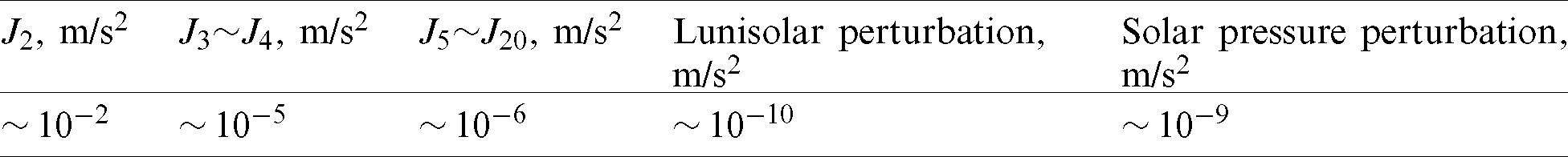
Assumption 1: The chaser is assumed to be a SEP spacecraft, whereas the target is a free-flying debris. Supposing the chaser or the debris is moving in a circular SSO with an altitude of approximately 800 km. The zonal harmonics perturbations up to 20 orders is considered only, because they are much significant than the other perturbations as shown in Tab. 1.

Assumption 2: The low thrust produced by electric propulsion is supposed to be directed to any direction without the change of thrust magnitude, which means that the maximum thrust available may keep constant during the entire transfer phase when the spacecraft is not in Earth shadow. This assumption is reasonable if the spacecraft’s solar panel may rotate at least in one-degree-of-freedom.

Assumption 3: Initial orbital states of the chaser and the target are supposed to be not widely spaced, wherein the semi-major axis, eccentricity, and inclination are constrained by the concept of the near-circular SSOs. The right ascension of ascending nodes (RAAN) are supposed to be similar whereas the phase angle difference between the chaser and the target can be arbitrary.

Table 1: Orders of the perturbing accelerations in a typical SSO

Assumption 4: The navigation error and the control error are not considered currently.

The third assumption implies that the chaser may rendezvous with the target in its neighboring orbit only. For a widely RAAN spaced rendezvous case, the reasonable strategy is to divide the entire flight into two phases: Minimizing orbital plane difference and orbital rendezvous, as shown in Fig. 1. The RAAN difference between the chaser and the target can be zeroed by adjusting the chaser’s orbital altitude, which leads to differential RAAN procession rate. Once the chaser reaches a target’s neighboring orbit, the phase for orbital rendezvous starts.

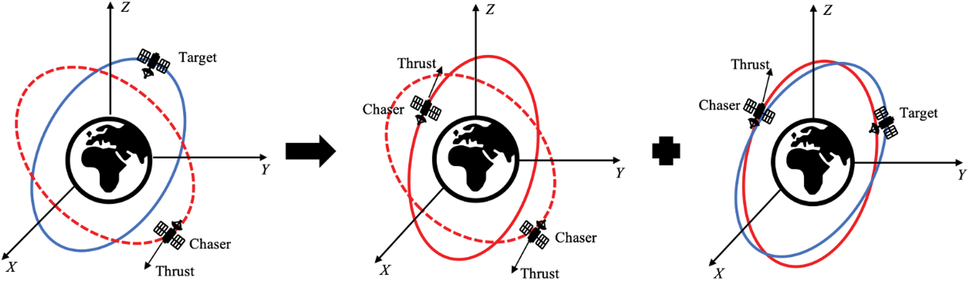
Figure 1: Illustration of two phases (left: widely spaced RAAN; middle: minimizing orbital plane difference; right: orbital rendezvous in this study)

2.2 Dynamic Equations

A set of non-singular modified equinoctial elements [27] (MEEs) 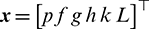is utilized to describe the states of the chaser and the target:

where a is the semi-major axis, e is the eccentricity, i is the inclination, is the RAAN, is the argument of periapsis, and is the true anomaly.

Let denotes the acceleration resulting from the natural perturbations and the active control, the perturbed Keplerian motion governed by Gauss’ variational equations can be written as

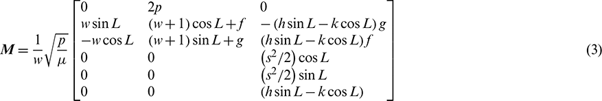
where is the gravitational parameter of the Earth, uR, uT, uN are the components of in the radial-transverse-normal (RTN) reference frame centered in the spacecraft, and , s2 = 1+h2+k2.

The acceleration in Eq. (2) consists of two parts: The perturbing acceleration from the natural perturbations and the active control acceleration

Based on Assumption 1 (Section 2.1), the perturbations considered in this study include zonal harmonics perturbations only. Because they are conservative force, Lagrange planetary equation [27] is adopted to compute the zonal harmonics perturbations instead of , that is

In addition, the thrust amplitude of the chaser, , satisfies

where is the maximum thrust amplitude available, L1 and L2 denote the exit and entry angles across the Earth shadow in each orbital revolution, respectively. Both L1 and L2 can be solved from the cylindrical Earth shadow model presented by [28]. Meanwhile, the unit direction vector of the thrust force satisfies

In this manner, the active control acceleration can be expressed as

where m is the spacecraft mass. The mass flow rate is expressed as

where is the specific impulse and is the gravitational acceleration at the sea level.

In Eq. (2), represents the two-body Keplerian motion, which leads the sixth element L to be a fast-changing variable. By contrast, the first five MEEs, p, f, g, h, k, are slow-changing variables defined as the following slow-changing vector

Then, the slow-changing vector is separated from the fast-changing variable to obtain . Considering that no active control is imposed on the target, the osculating orbital dynamics of the chaser and the target can be readily obtained as

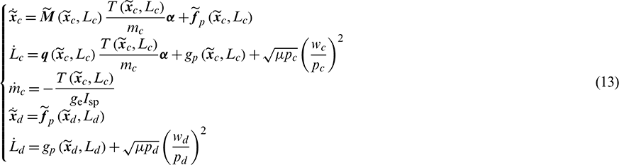
where the subscripts (c, d) represent the chaser and the target respectively, and

2.3 The LORP in SSOs

Assuming at the initial time t0, the state vectors of the chaser and the target are given by

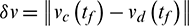
The LORP discussed in this study aims to provide an optimal control profile for the chaser, so that at a future time , the chaser reaches the target, i.e., satisfying

whereas the time of flight is minimized simultaneously. The motion of the chaser and the target are governed by the osculating orbital dynamics expressed in Eq. (13). For convenience, this LORP described in osculating elements is stated as Problem 1.

The description in Problem 1 is quite straightforward, but the problem is difficult to solve in reality because of the following two reasons. First, the practical thrust-to-weight ratio of the SEP spacecraft is generally small, which leads to a large number of orbital revolutions. As a result, direct numerical integration of Eq. (13) consumes an unacceptable amount of time during the numerical iteration for optimization. Second, the discontinuous thrust caused by Earth shadow is hard to formulate in an optimization problem using the osculating orbital dynamics Eq. (13). To avoid these difficulties, the orbital averaging technique is introduced in the following sections.

3  Optimal Control Problem Formulation Based on Orbital Averaging

3.1 Orbital Averaging

Referring to [9], by using the orbital averaging technique on Eq. (13), the averaged orbital dynamic equations can be obtained as:

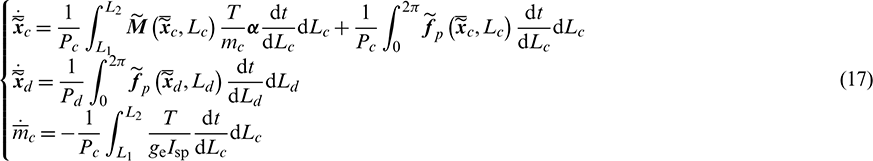
where a symbol denotes the averaged value of variable x and is the mean of the first five MEEs,

and

Similarly, as to the sixth element L, the mean longitude rate can be computed by

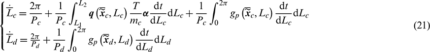
Defining as

which represents the mean longitude difference between the chaser and the target. Thus, the full averaged orbital dynamics of the LORP can be formulated as

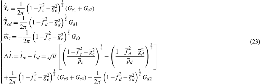
where

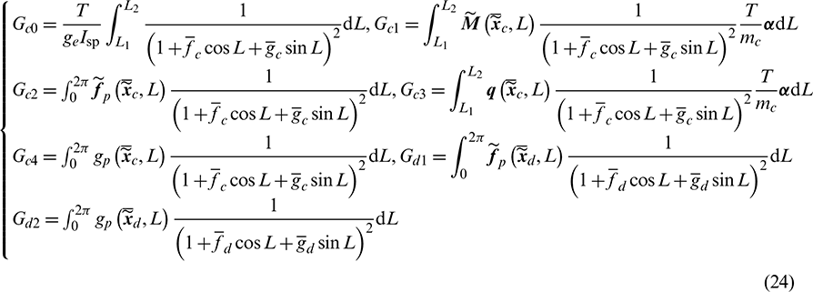
In this article, the averaged dynamic equations Eq. (23) are adopted to solve the optimal control problem for convenience. By using the orbital averaging technique, the discontinuous thrust caused by Earth shadow is easily handled by the definite integrals, which can be approximately computed by the numerical integration methods such as Gauss–Legendre quadrature. Moreover, all the mean elements on the left side of Eq. (23) change slowly and smoothly and the classical fourth-order Runge-Kutta method can be used for trajectory propagation.

3.2 Time Optimal Control Problem Formulation

Considering a time-optimal orbital rendezvous problem, the performance function is expressed as

Let 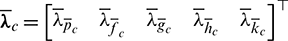, , be the costate variables (or Lagrange multipliers) associated with the state variables , , and , respectively. Based on the averaged orbital dynamic equation Eq. (23), the Hamiltonian function is defined as

The corresponding governing differential equations of costate variables can be written as

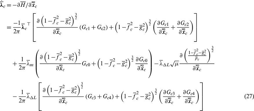
where the derivatives of are expressed as

According to Pontryagin’s maximum principle [29], the optimal control () is obtained if the Hamiltonian function takes the minimum, that is

where the admissible control domain is

Thus, the optimal thrust direction satisfies

while the optimal thrust amplitude should be maximum all the time, i.e.,

The specific solution of is attached in Appendix A. Consequently, if at the initial time t0, the initial conditions are known, the time-optimal orbital rendezvous problem can be transformed into a two-point boundary-value problem, defined as Problem 2 as follows:

Finding the specific value of the initial costate variables , , as well as the final time tf, such that the final states obtained by propagating the Eqs. (23) and (27)–(29) from t0 to tf can meet the necessary conditions, namely the terminal conditions

and the transversality conditions

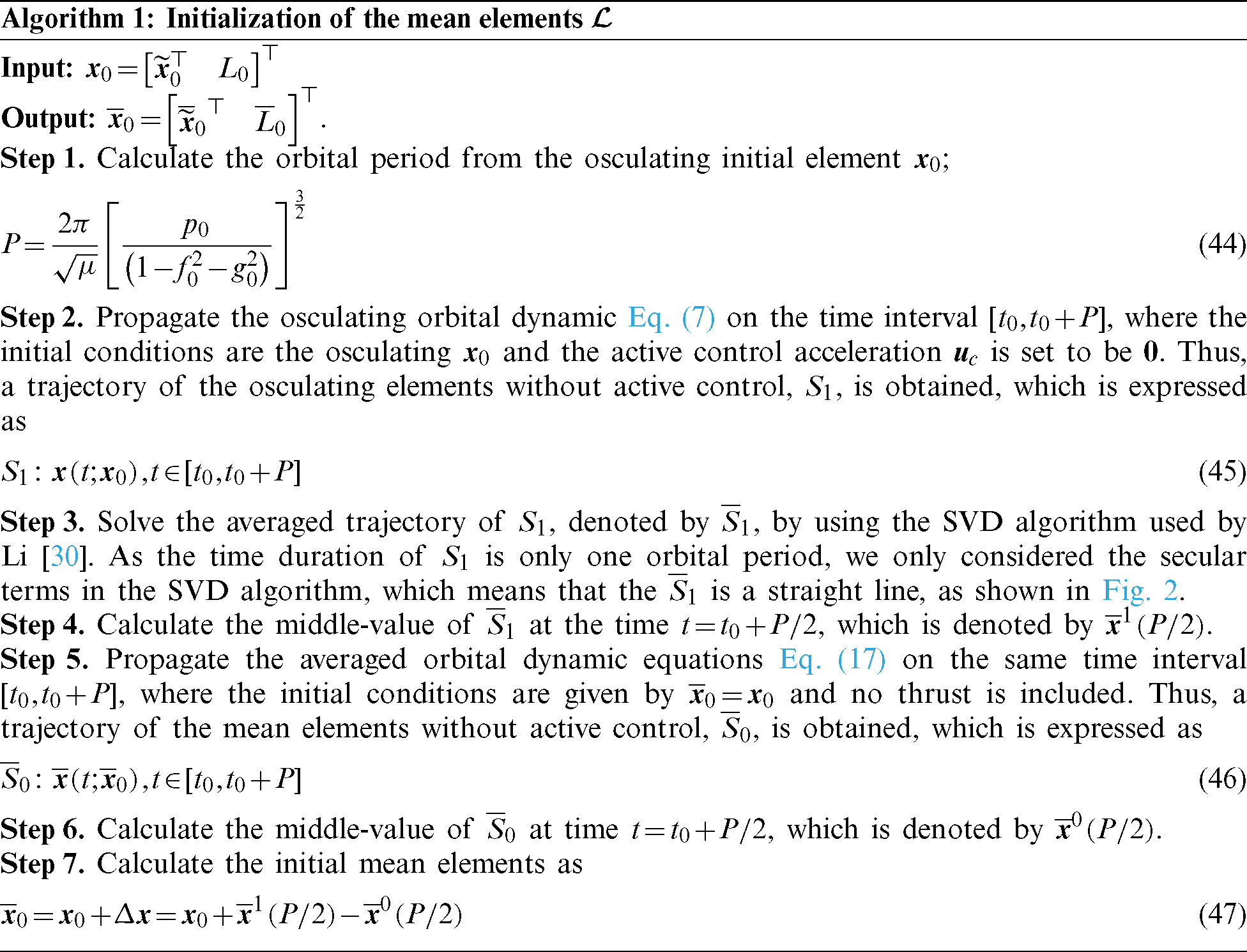
3.3 Initialization of the Mean Elements

The initial conditions of the chaser and the target are generally given in osculating MEEs by the navigation system, however, the averaged dynamic equation requires the mean elements , which should be transformed from the osculating elements . The transformation is based on the singular value decomposition (SVD) algorithm used by Li [30], where the algorithm is applied to find the mean elements for station-keeping of GEO satellites.

First of all, according to the osculating dynamic equation Eq. (13), is a piece-wise constant, which means that no short-term oscillation occurs for m. Thus,

Considering that the thrust-to-weight ratio of the chaser is much smaller than the zonal harmonics perturbations in SSOs, the effect of the active control can be reasonably neglected in a short time duration, for example only one orbital period. Thus, the elements’ transformations of the chaser are the same as that of the target. Let be the transformation, the details of are reported in Algorithm 1.

:

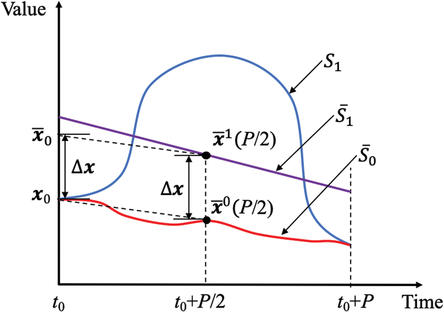
Figure 2: Initialization of mean elements using osculating elements

Until now, the initial mean , , and have been obtained. Finally, the initial mean is calculated from

In general, if is set positive, the chaser is leading the target initially, and if is set negative, the chaser is trailing the target initially. Therefore, a single rendezvous problem corresponds to two cases (leading or trailing) with or wherein .

4  Trajectory Optimization with the Averaged Orbital Dynamics

Problem 2 stated as a two-point boundary-value problem is still difficult to be solved directly using the shooting method because of the sensitivity of the initial costate variables. Thus, Problem 2 is transformed into the parameter optimization problem that is solved by taking advantages of mathematical programming solvers already developed and a series of practical techniques.

It is observed that the state equations Eq. (17), the costate equations Eq. (23), as well as the optimal control law in Eqs. (39) and (40) are all homogeneous with respect to the costate variables (or Lagrange multipliers) , except for the Hamiltonian function Eq. (26). Multiplying or dividing these multipliers by an arbitrary positive real number does not change the terminal states of the chaser and the target. Thus, if there are a set of Lagrange multipliers, whose initial value is , that satisfies Eq. (39) and

The necessary conditions left in Problem 2 can be easily achieved by multiplying a specific positive scaling factor, , that is

where C is the corresponding terminal value of the Hamiltonian function with respect to . The new Lagrange multipliers

are then the specific solutions of Problem 2, where all the necessary conditions involved are satisfied.

As a result, the approach for solving Problem 2 can be divided into two steps. First, the TPBVP is converted into a nonlinear programming problem (NLP), defined as Problem 3, where one of the transversality conditions, the equality constraint , is changed to an inequality constraint . Second, the specific scaling factor of the Lagrange multipliers is selected to satisfy the constraint . Problem 3 is totally equivalent to Problem 2, but the convergence domain is enlarged. Details of Problem 3 are summarized in Tab. 2.

Table 2: Nonlinear optimization model of Problem 3

The NLP is solved by sequential quadratic programming (SQP), which is a gradient based algorithm, and can be readily employed in many software tools. To improve the NLP convergence properties, the intelligent optimization algorithm, for example, the differential evolution (DE) [31] is employed to search good initial guesses. By using the normalization of the initial costate vector [32], the upper and lower bounds of the costate variables can be normalized to be [ −1,1]. As to the terminal time variable tf, the upper and lower bound can be estimated from the analytical phasing maneuver time [19] and the plane change time [24], and is obtained as follows:

where is the weighting function considering the Earth shadow, which represents the percentage of time the spacecraft is thrusting during one revolution:

Solving Problem 3 by both the DE and the SQP requires evolutions or iterations of optimization variables, and meanwhile propagating the state and costate equations. Owing to the use of orbital averaging, the computation complexity of such propagation is greatly simplified.

It is noted that DE usually costs much computational time to locate good initial guesses, while SQP obtains the converged solution much quickly if good initial guesses are available.

5  Trajectory Correction with the Osculating Orbital Dynamics

5.1 Control Law in Osculating Orbital Dynamic Equations

The optimal solution of orbital rendezvous is obtained in the solution space of mean elements. In the real mission, the osculating elements are obtained by the navigation system and considered to be the input to the control system. As a result, the optimal control profile expressed by mean elements needs to be transformed into the control law that steers the chaser using osculating elements.

First, the thrust amplitude, , satisfies

That is to say, the thrust keeps a maximum amplitude when the chaser is out of Earth shadow. The judgement of whether the chaser is in the shadow (the comparison between Lc and L1, L2) is tested continuously during the propagation.

As to the thrust direction, the most straightforward way is to take the optimal control profile in mean elements as the control law in osculating elements, with the phase angle L is replaced, i.e.,:

where L is the osculating phase angle and the mean costate variables , and the mean states involved are computed by the interpolation of , and that are optimization results from Problem 3. The thrust direction is only related to the osculating phase angle L, while , and are pre-stored quantities.

An alternative approach is that the control law of the chaser is governed by all the osculating elements. As indicated in Reference [33], the influence of thrust on the mean elements is approximated as that acting on the corresponding osculating elements. It is reasonable that the osculating elements and the mean elements are deemed the same to form the control law. Thus, the thrust direction profile in osculating elements is simply obtained by substituting into Eq. (39) for :

where the mean costate variables , are computed by interpolation of , . In this case, the thrust direction is depending on the osculating elements and L, while and are pre-stored quantities that can be deemed the gains for the control law.

As a result, once the Problem 3 is solved, the osculating trajectory of the chaser can be obtained by propagating the osculating orbital dynamic Eq. (13) from the initial time t0 to the final time tf, where the initial conditions are and the active control satisfies Eq. (54) and Eq. (55) or Eq. (56). Based on our experiences of solving a large number of numerical examples, the two strategies of the control law perform almost the same in precisely propagating the osculating orbital dynamic equations with the same set of initial states. This fact implies that the replacement of by is empirically acceptable, and the second strategy in Eq. (56) is more closely linked to the osculating elements that are obtained by the navigation system. It is noted that Zhong et al. [34] proposed an onboard mean-elements estimator, but it is not used in this study and our experiences show that Eq. (56) makes the control law effective and simpler.

5.2 Accuracy Verification and Error Correction Strategy

When we numerically propagated the orbital dynamic equations expressed by osculating elements with the control laws in Eqs. (54) and (56) obtained by solving Problem 3, we found that the terminal orbital rendezvous errors exist, namely the terminal states of the chaser may not precisely meet those of the target. These errors stem from a series of approximations, as listed in Tab. 3.

Table 3: List of approximations

It is found that the most significant rendezvous error is the difference in the true longitude between the chaser and the target at the terminal time. Considering the true longitude L is a fast-changing variable, a correction about the initial mean longitude difference can effectively compensate for the rendezvous errors. Let be the correction factor, which is a single scalar; and 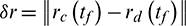, be the terminal position and velocity errors between the chaser and the target in osculating elements, the correction of the initial mean longitude difference is expressed as

As a result, the new problem is proposed, that is: finding the optimal that contributes to the minimum of objective function

where and are the weight coefficients and are configured according to different emphasis on the terminal position and velocity errors. The optimization interval of is chosen as [ −0.15,0.15] empirically, which means a slight correction of plays an important role in eliminating the terminal rendezvous errors. This univariate optimization problem is readily solved by many mature numerical methods, such as the Golden section search and the Fibonacci search [35]. For convenience, this strategy is termed -correction in this work.

During the process of -correction, there are two layers of optimization iterations. The outer iteration is the univariate optimization with respect to , and the inner iteration is the NLP optimization (solving Problem 3) with the initial conditions changed (related to ), which can be readily solved by SQP from the solution with the initial conditions be , where . When J+ reaches its minimum, Problem 3 is solved to obtain the optimal control in the solution space of mean elements and orbital accuracy of the control laws is also met with osculating elements. In this study, the orbital rendezvous is deemed to be achieved if J+ is small enough.

The -correction perturbs the initial and leads to adjustment of the costate variables or the gains of control law. This strategy can be applicable to other mean elements if necessary. Although empirical, it is effective for solving concerning problems, which is validated by several hundreds of examples shown in Section 6.

6  Numerical Example

In this section, two typical LORP examples in SSOs are provided in details, namely: (1) The quasi phasing maneuver problem and (2) The general LORP. In example (1), the first five MEEs of the chaser and the target are nearly the same initially, the chaser mainly implements the phasing maneuvers; in Example (2), the chaser and the target differs in the semi-major axis (100 km difference) and the phase location at the initial time. More examples are tested via continuation of the chaser’s initial states, which generated several hundreds of examples to validate the proposed method.

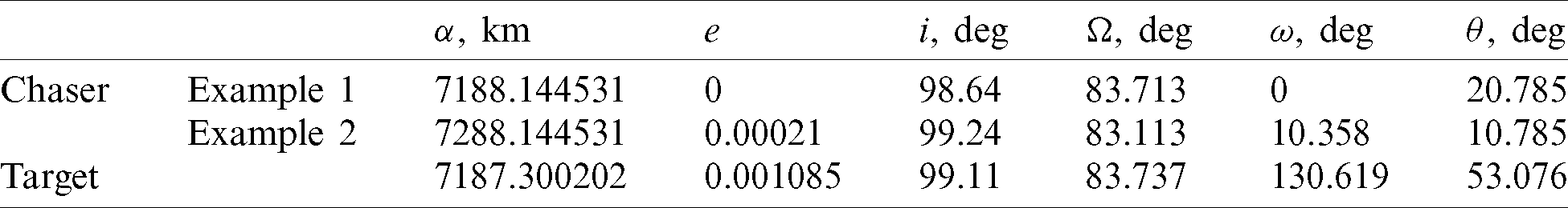
For simplicity, the initial time epoch is set at January 1, 2025, 00:00:00.000 UTCG for all simulation examples. The target is chosen as a real free-flying debris moving in an SSO, whose DISCOS ID is 23753. It is a rocket mission related object and the size is larger than 5 m2 [36]. The orbital states of the target at the initial time epoch can be obtained via the SGP4 propagation model. The chaser, a servicing SEP spacecraft, is supposed to be injected into a nearby orbit with the initial mass and the thruster’s configuration presented in Tab. 4. The low thrust produced by electric propulsion is supposed to be directed to any direction and the maximum thrust available keeps constant during the entire transfer phase. The initial states, in terms of the classic orbital elements under the J2000 inertial frame, of the chaser and the target, are given in Tab. 5. The perturbations include the zonal harmonics of the non-spherical Earth gravitational perturbations up to 20 orders of the EGM96.

Table 4: Configuration of the chaser

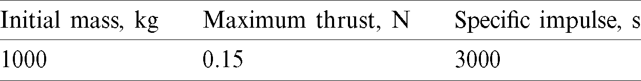
Table 5: Initial classical orbital elements of the chaser and the target

As mentioned before in the initialization of the mean elements (Section 3.3), there are two cases for a rendezvous problem: leading and trailing, wherein is set positive and negative separately. It is uncertain in advance that the transfer time of which case will be shorter, as a result, in the following examples, both cases were solved. The integral interval for propagating the averaged dynamic equations is set as revolutions, and the integral precision adopted to calculate the terminal errors in osculating elements by propagating the osculating dynamic equations is defined by a relative error tolerance of and an absolute error tolerance of . The weight coefficients and are both set to be 1 to just weight the terminal errors and equally. Meanwhile, the stopping criteria of the univariate optimization for -correction is set to be . During the computation, all the unit of the range and velocity are normalized by Earth’s radius Re and separately to get a better convergence.

6.1 Example 1: Quasi Phasing Maneuver Problem

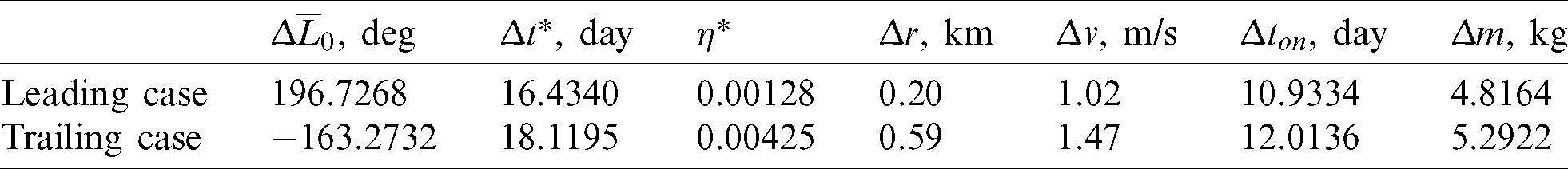
In this example, the chaser and the target are supposed to be located in nearby SSOs with the orbital altitudes of around 810 km. When Problem 3 is solved and the -correction is made, the solutions of the leading case and trailing case are summarized in Tab. 6.

Table 6: Solutions of Example 1

where is the optimal correction factor, is the minimum flight time, and represent the corresponding terminal differences of position and velocity after correction, respectively. In addition, and denote the working time of the thruster and the fuel consumption during the maneuver. It shows that the trailing case results in a shorter flight time, thus, the trailing case is discussed further below.

The time history of the osculating and mean MEEs (p, f, g, h, k) and the longitude difference are shown in Fig. 3. These results show that the chaser gradually approaches the target. In addition, the entire maneuver turns out to be a “catch-up” process, as the phase difference increases from negative to 0 monotonically.

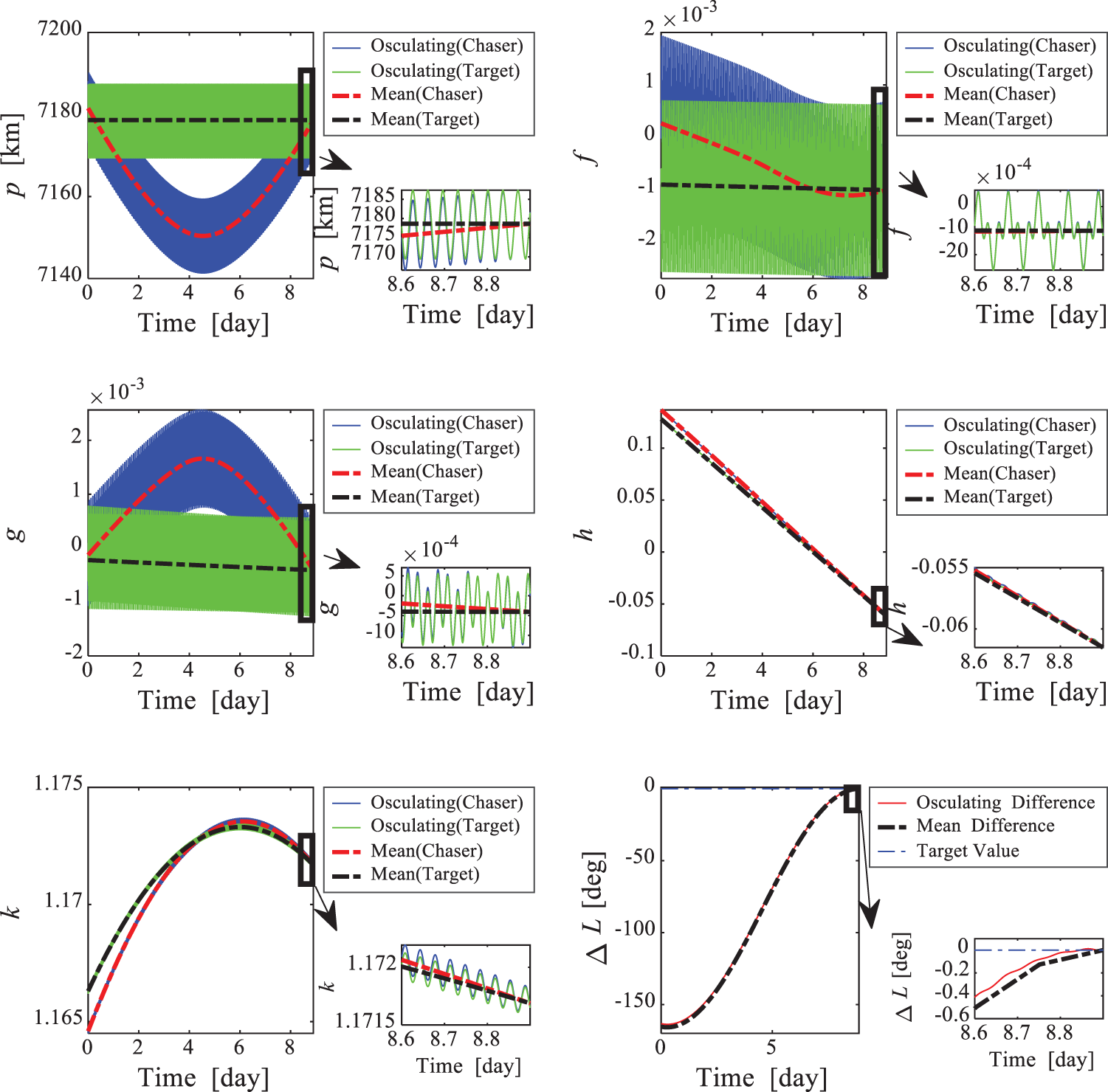
Figure 3: Evolutions of p, f, g, h, k, in Example 1

The time histories of the thrust direction under the RTN reference frame are presented in Fig. 4. It shows that the thrust direction changes periodically along the transfer phase. At the first half transfer, the component of the thrust is negative, thus, decreasing the semi-major axis to catch up with the phase; while at the second half, it turns to positive to increase the semi-major axis to the desired target value. The component of the thrust keeps a relative high value to compensate for the orbital plane change throughout the flight as the change of semi-major axis leads to a continuous drift difference of RAAN between the chaser and the target. In addition, the component of the thrust is imposed mainly at the middle part of the maneuver.

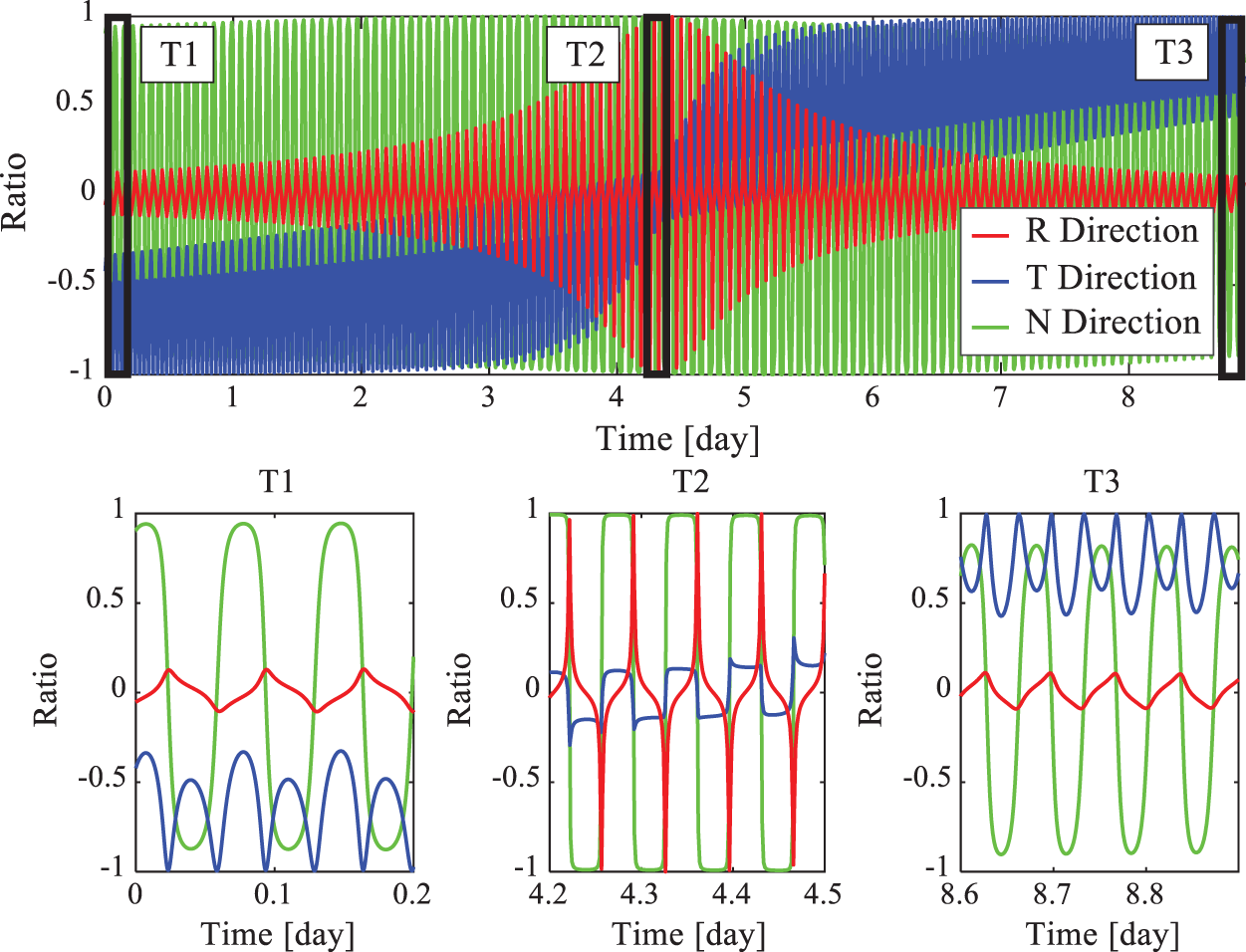
Figure 4: History of the control direction under RTN reference frame in Example 1

Under the J2000 inertial frame, trajectories of the chaser and the target are shown in Fig. 5. At the initial time, the chaser and the target are located at the points represented by the black and green dots, respectively. At the final time, terminal positions of the chaser and the target are denoted by the black triangle and green pentagon. The overlapping of the terminal positions indicates that the chaser rendezvouses with the target. The chaser passes the Earth shadow in each revolution, as the blue lines represent the chaser enters the shadow in which the thruster is off. The total number of the complete revolutions for the chaser to rendezvous with the target is 127.

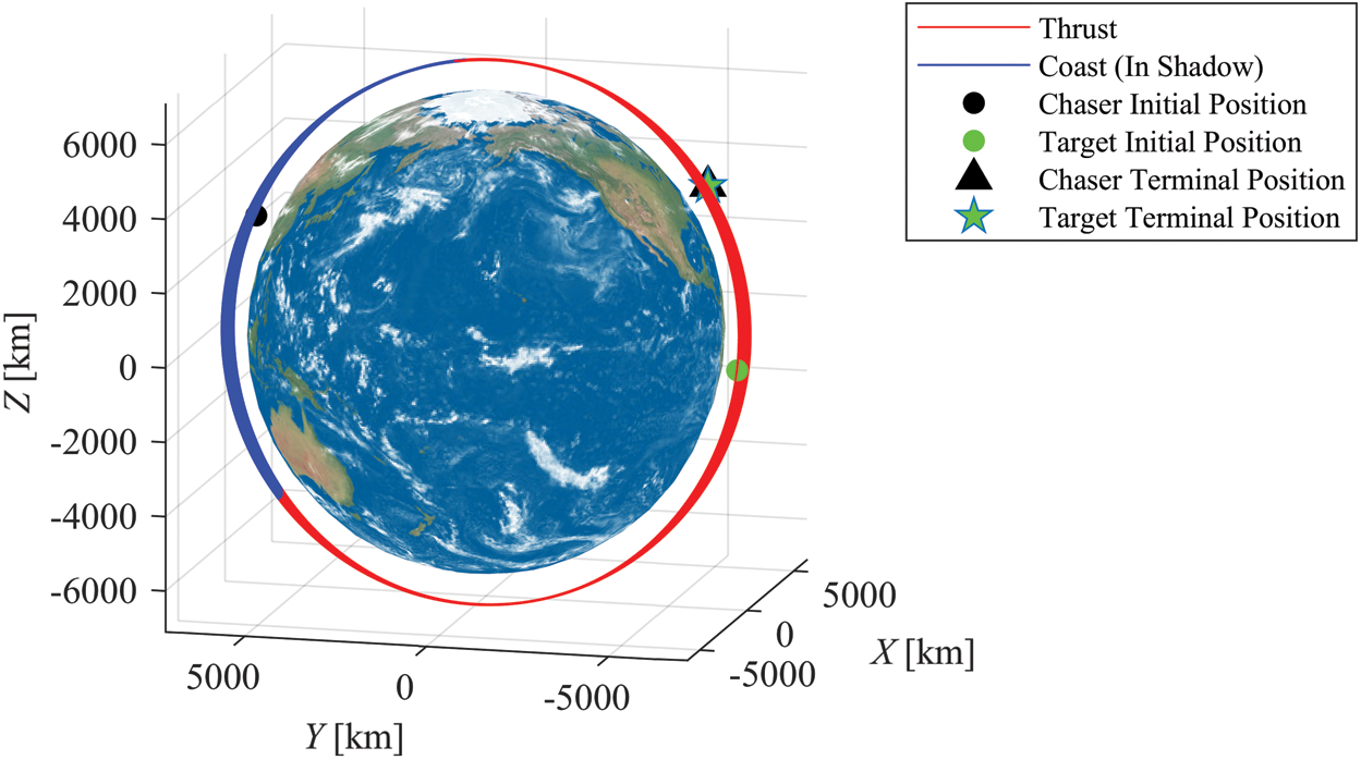
Figure 5: Trajectories of the chaser for the rendezvous in Example 1

6.2 Example 2: General LORP

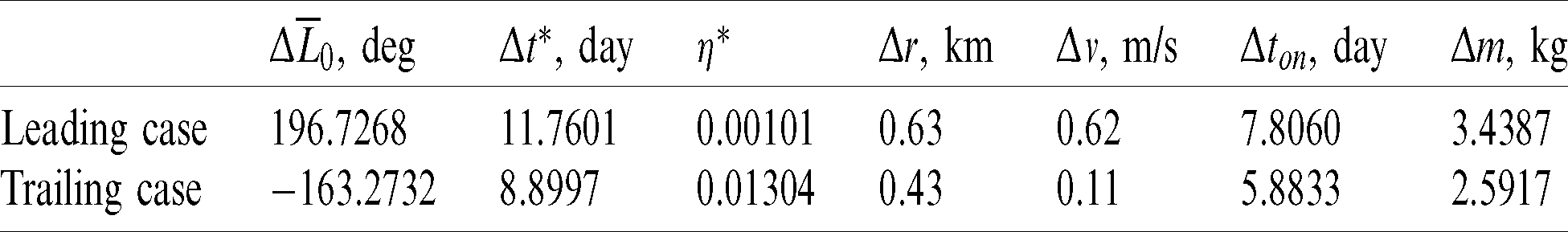
In this example, the chaser and the target are supposed to be located in SSOs with the altitude of 900 km and 810 km separately. When Problem 3 is solved and the -correction is made, the solutions of the leading case and trailing case are summarized in Tab. 7. Different from Example 1, the leading case in Example 2 takes a better result, which is discussed further below.

Table 7: Solutions of Example 2

The time history of the osculating and mean MEEs (p, f, g, h, k) and the longitude difference are shown in Fig. 6. The entire maneuver turns out to be a process including both “waiting-for” and “catch-up,” as the phase difference changes from positive to negative and eventually to 0.

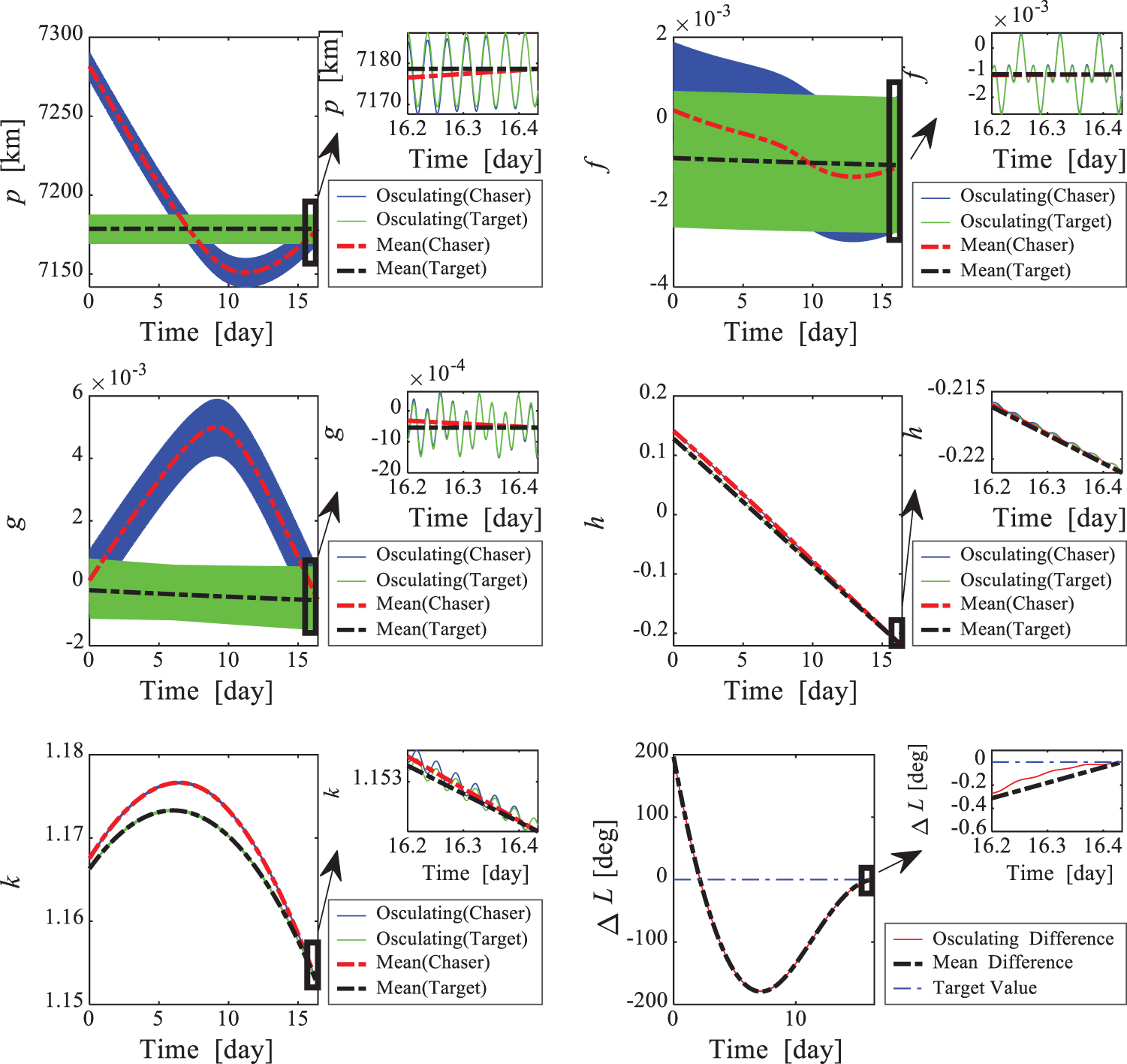
Figure 6: Evolutions of p, f, g, h, k, in Example 2

The time histories of the thrust direction under the RTN reference frame are presented in Fig. 7. The thrust direction during the rendezvous still displays a periodic change along the transfer phase, but the whole evolution is quite different with that in Example 1. The sign of the component is not exactly changed at the half and the component is imposed mainly at the end part. Moreover, the component is small at the beginning while in the later, the proportion is large where the main plane change is conducted.

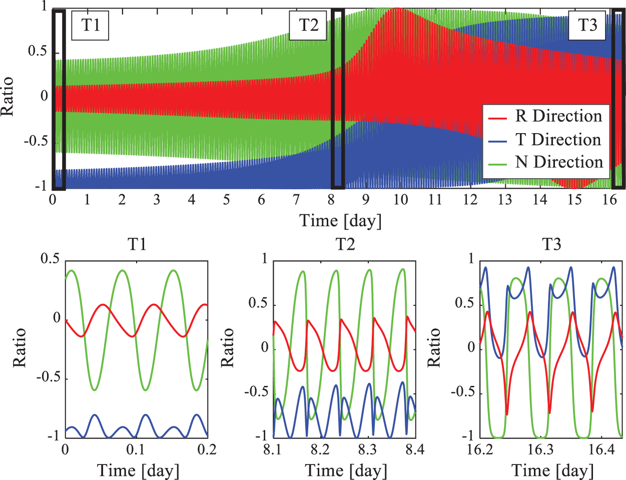
Figure 7: History of the control direction under RTN reference frame in Example 2

Under the J2000 inertial frame, trajectories of the chaser and target are shown in Fig. 8. The total number of complete revolutions for the chaser to rendezvous with the target is 234.

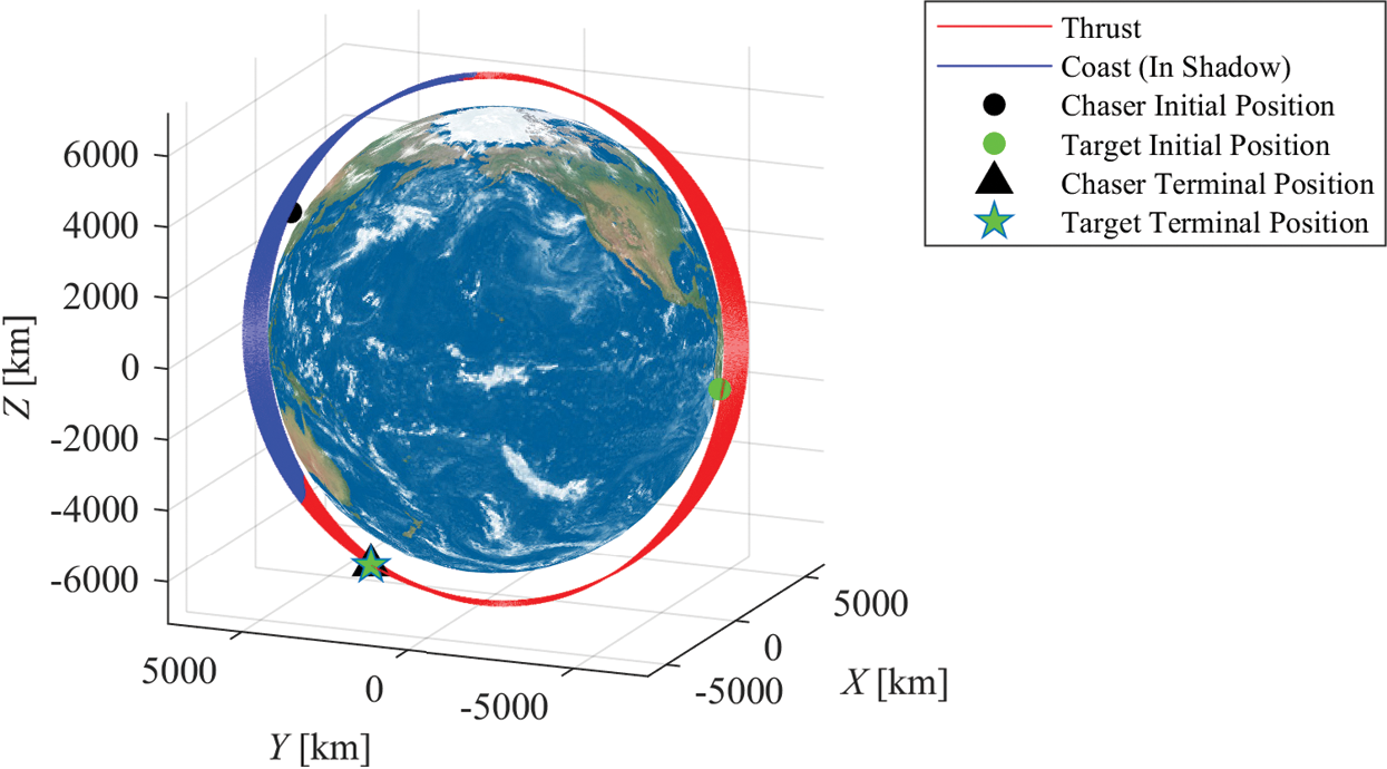
Figure 8: Trajectories of the chaser for the rendezvous in Example 2

6.3 Continuation of the Initial States of the Chaser

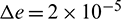
In this subsection, more examples are tested to verify the correction strategy numerically. Considering it is time-consuming to do the Monto-Carlo simulation because of the DE involved in solving Problem 3, the continuation method is adopted instead. The parameter of the continuation is set to be the chaser’s initial orbital states, namely a, e, i, and , whereas the target remains unchanged. The starting point of the continuation is the same with the chaser’s initial states stated in Example 1. Figs. 9 and 10 show the minimum rendezvous time obtained, and the intervals between the discrete points (i.e., the continuation step) are set as , , , , seperately.

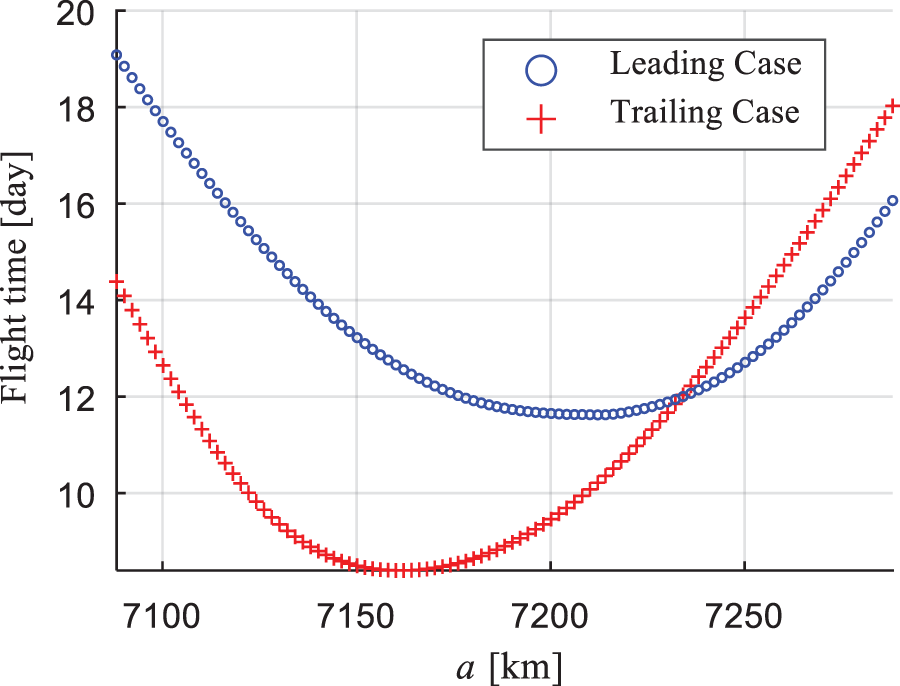
Figure 9: Continuation on a

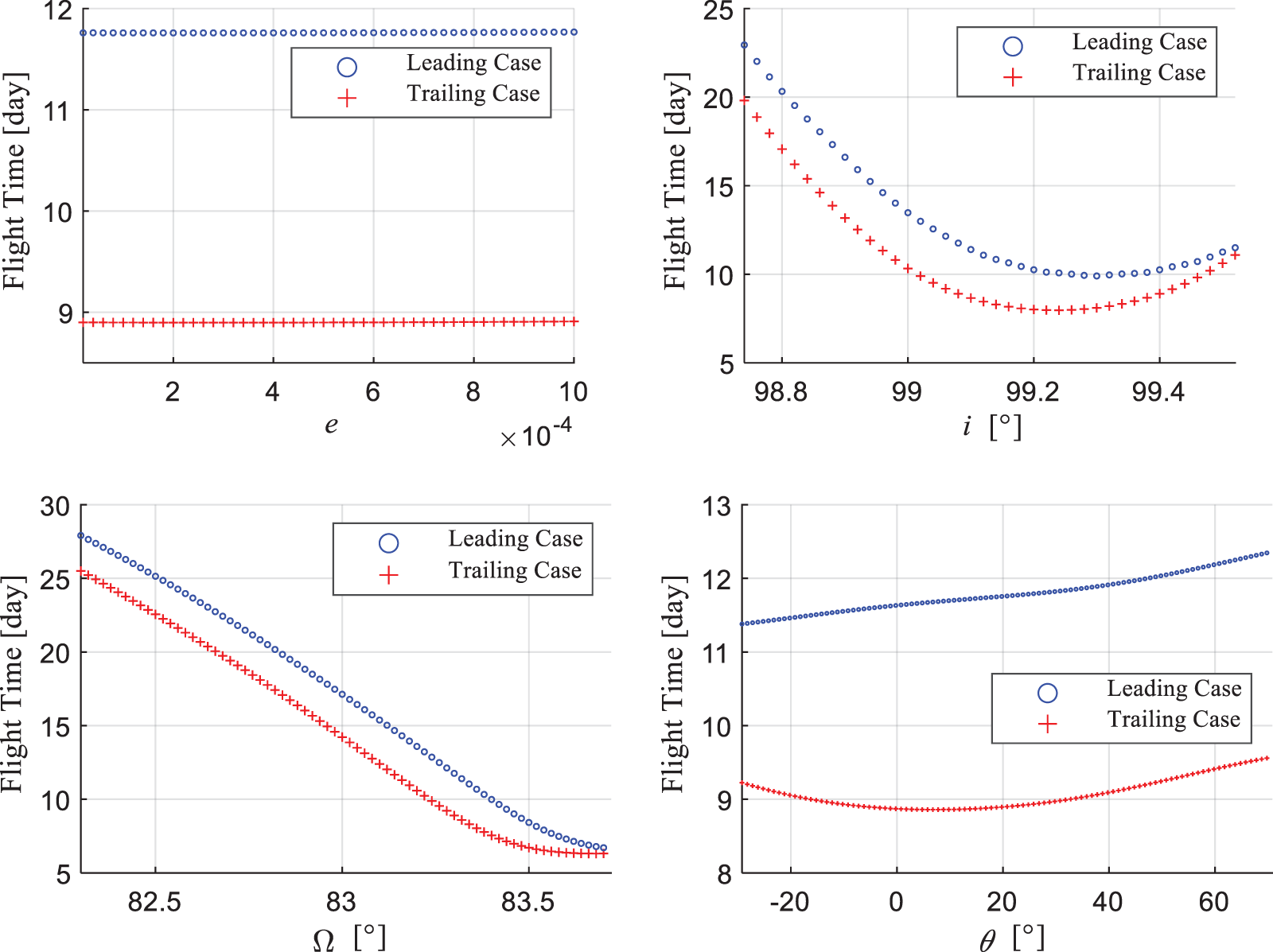
Figure 10: Continuation on

Obviously, when the initial states of the chaser changed, the resulting difference of both orbital plane and orbital size lead to a different minimum rendezvous time. The red dots represent the leading case, whereas the blue represent the trailing case. The cross point between the blue line and red line in Fig. 9 indicates that at this specific point the minimum rendezvous time of both cases meet a same result, whereas the transfer orbits are totally different. In addition, compared to other elements, the change of eccentricity (nearly zero) has little effect on the minimum rendezvous time.

The continuation generates 750 examples. The flight time correction and correction factors for all these examples are summarized in Fig. 11, showing that the resulting changes of the flight time are less than 0.2 day, which is no more than 3 revolutions compared to the total revolutions up to hundreds. Tab. 8 represents the statistics of , demonstrating that the corrections made are relatively slight. In addition, as shown in Fig. 12, the terminal orbital errors in position and velocity can be reduced to the order of 1 km and 1 m/s simultaneously, which are acceptable by the relative navigation system. The -correction strategy, which is empirical but simple, demonstrates its effectiveness to generate the control laws that precisely steer the chaser to the target.

Figure 11: Flight time correction and correction factors during the continuation

Table 8: Statistics of correction factors

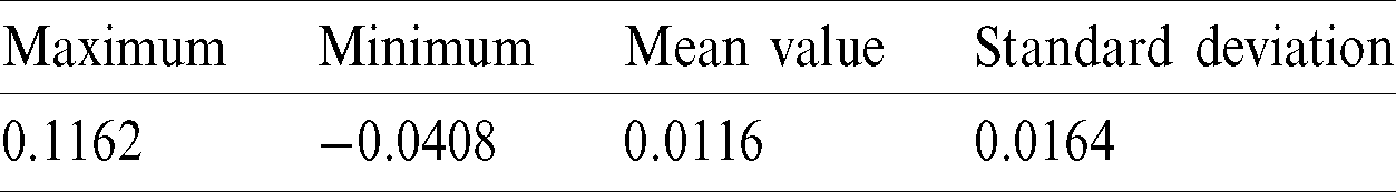
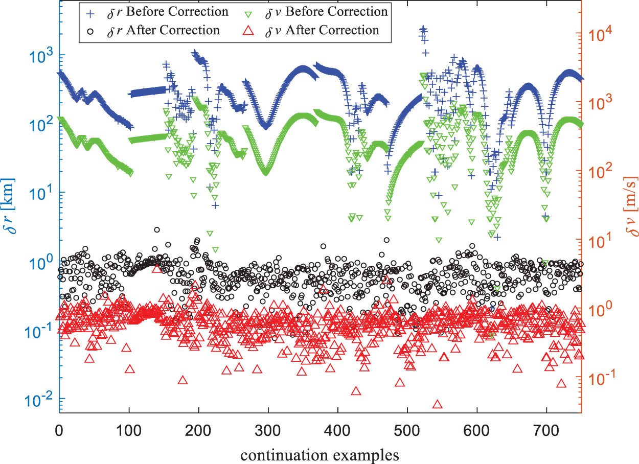
Figure 12: Terminal errors before and after correction

7  Conclusions

Considering the prospect of the solar electric propulsion spacecraft for debris removal missions, a practical optimization method is proposed to compute the optimal low-thrust minimum-time many-revolution orbital rendezvous in sun-synchronous orbits, which usually consists of a large number of ballistic orbital arcs in Earth shadow. Different from the existing works, the prominent advantage of the proposed method are twofold: (1) The orbital averaging technique is used with a new slowing-changing variable (the mean longitude difference) proposed to accommodate to the rendezvous problem, which makes it easily to model the perturbations and thrust discontinuity in Earth shadow, and the computational complexity is greatly simplified in the aspect of numerical iterations for trajectory optimization. (2) By using a simple correction strategy, the resulting optimal control derived from the mean orbital dynamics and the corresponding costate variables is mapped to the control law that is used in osculating orbital dynamics to guarantee the rendezvous describing in osculating elements. The effectiveness of the proposed optimization method was successfully demonstrated by two typical low-thrust-orbit-rendezvous missions and hundreds of running with the continuation of the initial states.

Funding Statement: This work was supported by the National Key Research and Development Project (Grant No. 2018YFB1900605) and the Key Research Program of Chinese Academy of Sciences (Grant No. ZDRW-KT-2019-1).

Conflicts of Interest: The authors declare that they have no conflicts of interest to report regarding the present study.

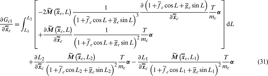
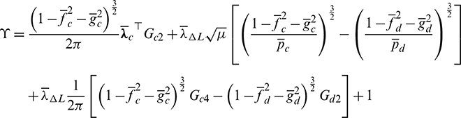
Appendix A: Deduction of Optimal Control Substituting Eq. (23) into Eq. (26), the Hamiltonian function can be rewritten as

where is the specific items related to the active control . The expressions of and are

were

It is observed that

Thus, to minimize , should be minimized, resulting to that the optimal unit direction vector is opposite to the vector , i.e., satisfies

Substituting the optimal thrust direction into Eq. (28), it is readily to obtain . Meanwhile, the terminal costate of the mass satisfies the transversality condition . Thus, is a non-negative real number during the entire transfer phase. In addition, substituting into , the coefficient before T is rewritten as

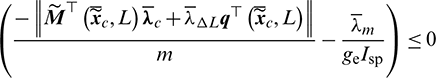
which is a non-positive real number. As a result, the optimal thrust amplitude should be maximum all the time, i.e.,:

This work is licensed under a Creative Commons Attribution 4.0 International License, which permits unrestricted use, distribution, and reproduction in any medium, provided the original work is properly cited.