Computer Modeling in Engineering & Sciences

DOI: 10.32604/cmes.2021.013206

ARTICLE

Stability and Bifurcation of a Prey-Predator System with Additional Food and Two Discrete Delays

Ankit Kumar and Balram Dubey*

Department of Mathematics, BITS Pilani, Pilani Campus, Pilani, 333031, India
*Corresponding Author: Balram Dubey. Email: bdubey@pilani.bits-pilani.ac.in
Received: 29 July 2020; Accepted: 22 October 2020

1  Introduction

Living organisms on the surface of the earth adopt only the way that boosts their survival possibilities so that they can pass their genes to the next generation. There are several fundamental instincts in ecological communities and, predation is one of them that constitutes the building blocks for multispecies food webs. Initially, Lotka [1] and Volterra [2] studied the model for prey-predator interaction and observed the uniform fluctuations in the time series of the system. On later the fluctuations were removed from the system by taking logistic growth of prey population [3,4]. Many researchers have widely studied prey-predator interactions for the last century [5–12]. They have considered several essential concepts over time that play a vital role in the dynamics of the system like functional response, time delay, harvesting and conservation policies of species, stage structure, fear induced by predators, etc. The idea of functional response was proposed by Holling [5]. It is defined as the consumption rate of prey by predators. Holling considered it nonlinear function of prey species that saturates at a level. Further, it was considered a function of prey and predator both by several authors [6,10,13,14].

In last few decades, many authors have studied the qualitative dynamics of prey-predator systems in the presence of additional food resources for predators [15–20]. Additional food is an important component for predators like coccinellid which shapes the life history of many predator species [17]. Ghosh et al. [20] investigated the impact of additional food for predator on the dynamics of prey-predator model with prey refuge and they observed that predator extinction possibility in high prey refuge may be removed by providing additional food to predators. Again, to study the role of additional food in an eco-epidemiological system, a model was proposed and studied by Sahoo [21]. The author found that the system becomes disease free in presence of suitable additional food provided to predator. Recently, a prey-predator model with harvesting and additional food is analyzed by Rani et al. [22] and they have shown some local and global bifurcation with respect to different parameters. To incorporate the additional food into the model, they modified the Holling type II functional response.

Delayed models exhibit much more realistic dynamics than non delayed models [4,23]. In prey-predator system, the impact of consumed prey individuals into predator population does not appear immediately after the predation, there is some time lag that is gestation delay [24]. We incorporate the effect of time delay into the model with delay differential equations. A delay differential equation demonstrates much more complex character than ordinary differential equation. On the other hand predators do not consume the additional food as soon as it is provided. They take some time to consume and digest the food. Delayed models are widely studied by researchers [10,14,25–33]. A delayed prey and predator density dependent system is investigated by Li et al. [10]. The authors analyzed stability, Hopf-bifurcation and its qualititative properties by using Poincare normal form and the formulae given in Hassard et al. [34]. Sahoo et al. [35] examined prey-predator model with effects of supplying additional food to predators in a gestation delay induced prey-predator system and habitat complexity. They have pointed out that Hopf-bifurcation occurs in the system when delay crosses a threshold value that strongly depends on quality and quantity of supplied additional food. The effect of additional food along with fear induced by predators and gestation delay is discussed by Mondal et al. [36]. There are several studies carried out with multiple delays [37–40]. Li et al. [37] have done stability and Hopf-bifurcation analysis of a prey-predator model with two maturation delays. Gakkhar et al. [30] explored the complex dynamics of a prey-predator system with multiple delays. They established the presence of periodic orbits via Hopf-bifurcation with respect to both delays. Recently, Kundu et al. [40] have discussed about the dynamics of two prey and one predator system with cooperation among preys against predators incorporating three discrete delays. The authors have found that all delays are capable to destabilize the system.

To the best of our knowledge, an ecological model including (i) Effect of additional food supplies to predators, (ii) Dependency factor of supplied additional food, (iii) Holling Type II functional response, (iv) Gestation delay in predator have not been considered. Inspired by this, we establish three dimensional non delayed and delayed models in Section 2. We analyze the dynamics of non delayed model and validate it via some numerical simulations in Section 3. In Section 4, we analyze the dynamics of delayed model through Hopf-bifurcation. Direction and stability of Hopf-bifurcation are carried out in Section 5. Section 6 is devoted to the numerical simulations for delayed model. Conclusions and significance of this work are discussed briefly in Section 7.

2  Proposed Mathematical Model

We consider a habitat where two biological populations, prey population and predator population are surviving and interacting with each other. It is assumed that prey population grows logistically and the interaction between prey and predator follows Holling Type II functional response. We assume that the density of the additional food supplied to the predators is directly proportional to the density of predators present in the habitat. Keeping these in view, the dynamics of the system can be governed by the following system of differential equations:

In the above model x(t), y(t) are number of prey and predator individuals at time t and A is quantity of additional food provided to predators. A0 is dependency factor of predators on provided additional food resources. If A0 = 1, then predators depend completely on additional food and prey population grows logistically. If A0 = 0, then predators depend only on the prey population and in such a case additional food is not required. is maximum supply rate of additional food resources.

In real situations, each organism needs an amount of time to reproduce their progeny. Due to this fact the increment in predators does not appear immediately after consuming prey. It is assumed that a predator individual takes time for gestation. Therefore, it seems reasonable to incorporate a gestation delay in the system. Thus, the delay is considered in the numeric response only. Again it is assumed that the additional food is provided to predators with another delay . The generalized model involving these two discrete delays takes the following form

subject to the non negative conditions , , where and , (i = 1, 2, 3).

The biological meaning of all parameters and variables in above models is provided in Tab. 1.

Table 1: Variables and parameters used in Models (1) & (2)

3  Dynamics of Non-delayed Model

First of all, we examine the boundedness and persistence of the system (1).

3.1 Boundedness and Persistence of the Solution

Theorem 3.1. The set

is a positive invariant set for all the solutions of model (1), initiating in the interior of the positive octant, where .

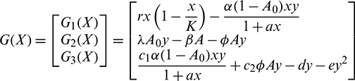
Proof The model system (1) can be written in the matrix form

where and G(X) is given by

Since is locally Lipschitz-continuous in and the fundamental theorem of ordinary differential equation guarantees the local existence and uniqueness of the solution. Since , it follows that for all . In fact, from the first equation of model (1), it can easily be seen that , and hence , for all . Secondly, for all (as for all .) and hence for all

From the first equation of model (1), we can write

which yields

Now, suppose

then we have

where

Hence, it follows that

We also note that if and 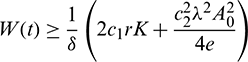, then , . This shows that all solutions of system (1) are bounded and remains in for all t > 0 if

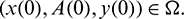
Theorem 3.2. Let the following inequalities are satisfied:

Then model system (1) is uniformly persistence, where, xa is defined in the proof.

Proof: System (1) is said to be permanence or uniform persistence if there are positive constants M1 and M2 such that each positive solution X(t) = (x(t), A(t), y(t)) of the system with positive initial conditions satisfies

Keeping the above in view, if we define

then from Theorem 3.1, it follows that

This also shows that for any sufficiently small , there exists a T > 0 such that for all , the following holds:

Now from the first equation of model system (1), for all , we can write

Hence, it follows that

which is true for every , thus

where

Now from the third equation of model system (1), we obtain

which implies

which is true for every , thus

for persistence, we must have .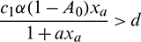

Second equation of model system (1) yields

Hence

Taking 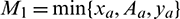, the theorem follows.

Remark. Theorem 3.2 shows that threshold values for the persistence of the system are dependent on the parameter A0.

3.2 Equilibrium Points and Their Stability Behavior

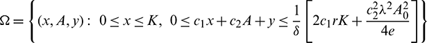
System (1) has four equilibrium points, trivial equilibrium E0(0, 0, 0), axial equilibrium E1(K, 0, 0), prey free equilibrium and interior equilibrium E*(x*, A*, y*). E0 and E1 always exist.

1.    Existence of : The prey free equilibrium E2 is positive solution of the following system:

From the second equation of above system, we have

Putting the value of A in the first equation of system (3), we get

Above equation has two positive roots if

System (1) has two prey free equilibrium under conditions given in (5): and . Again, If 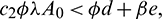then Eq. (4) does not have any positive root. Therefore, E2 does not exist in this case.

2.    Existence of interior equilibrium E*(x*, A*, y*): It may be seen that x*, A* and y* are the positive solution of the following system of algebraic equations:

From the second equation of system (6), we have

Putting this into the first and third equation of system (6), we obtain the following system:

We note the following points from Eq. (7):

1.    When y = 0, then 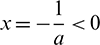or x = K > 0.

2.    When x = 0 then .

3.    

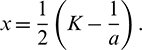
Similarly, from Eq. (8), we note the following:

1.    When y = 0, then

2.    

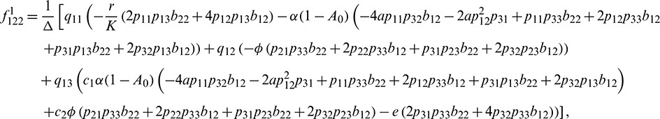
From above analysis we can conclude that system (6) has a unique positive solution (x*, A*, y*) if, in addition to condition (9), the following holds:

Hence, we can state the following theorem.

Theorem 3.3. The system (1) has a unique positive equilibrium E*(x*, A*, y*) if (9) and (10) hold.

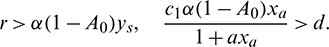
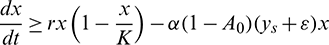
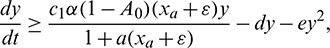
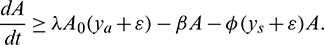
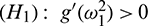
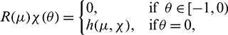
Remark. The number of positive equilibrium for the system (1) depends on values of parameters, which we have chosen. Several possibilities are depicted in Fig. 1.

Figure 1: Four possibilities of the prey and predator zero growth isoclines. (a) Interior equilibrium does not exist for the parametric values a = 0.08, d = 0.01, (b) interior equilibrium exists uniquely for the values of parameters a = 0.1, d = 0.235, (c) two interior equilibria for parameter values a = 0.1, d = 0.137, (d) three interior equilibria for parameter values a = 0.105, d = 0.1. Rest of the parameters are same as that in (25)

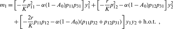
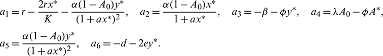
The local behavior of a system in the vicinity of any existing equilibrium is very close to the behavior of its Jacobian system. So, we compute the Jacobian matrix to see the local behavior of the system around its equilibrium and we observe that

•    The trivial equilibrium E0(0, 0, 0) is always a saddle point having stable manifold along the A and y-axes and unstable manifold along the x-axis.

•    The axial equilibrium E1(K, 0, 0) is locally asymptotically stable if . If , then E1 is a saddle point having stable manifold along the x and A-axes and unstable manifold along the y-axis.

•    The Jacobian matrix evaluated at prey free equilibrium is given by

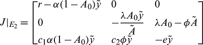
Characteristic equation is given by

The roots of Eq. (11) have negative real part if

Hence is asymptotically stable under condition (12).

Eq. (11) have at least one positive and one negative root if

Therefore, is a saddle point under condition (13).

Remark. By replacing by and by similar analysis holds good for the stability behavior of

•    In order to analyze the local stability of unique interior equilibrium E*(x*, A*, y*), we evaluate the Jacobian matrix at E* and it is given by

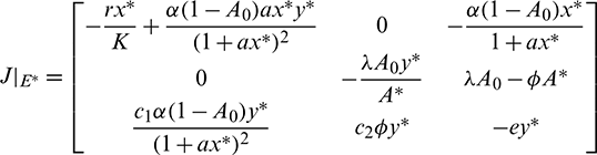
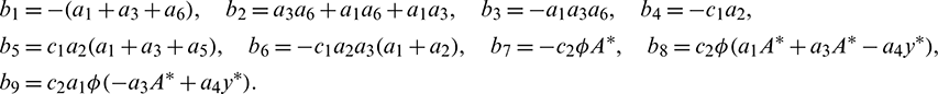
Characteristic equation corresponding to above matrix is given by

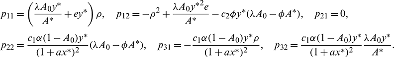
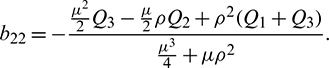
where

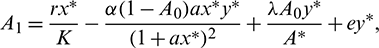
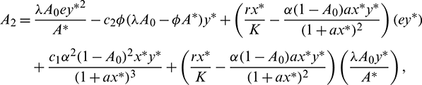
Now using the Routh–Hurwitz criterion, all eigenvalues of J|E* have negative real part iff

Thus we can state the following theorem.

Theorem 3.4 The system (1) is stable in the neighborhood of its positive equilibrium iff inequalities in (15) hold.

It is also noted that inequalities in (15) hold if

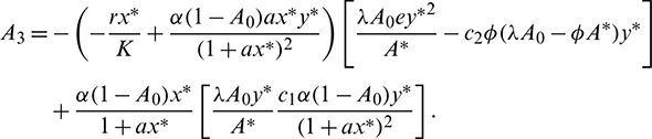
Infect, the above two conditions imply that A1 > 0 and A3 > 0. The third condition A1A2 > A3 is also satisfied.

Remark. The system (1) is stable around its positive equilibrium E* if inequalities in (16) hold.

In the following theorem we give a criterion for global asymptotic stability of interior equilibrium E*(x*, A*, y*) of the system (1).

Theorem 3.5. The interior equilibrium E*(x*, A*, y*) of the system (1) is globally asymptotically stable under the following conditions:

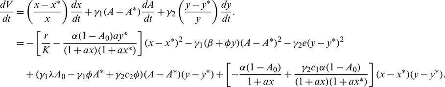
Proof. We Choose a suitable Lyapunov function about E* as

where and are positive constants, to be specified later. Now, differentiating V with respect to t along the solutions of system (1), we get

Choosing 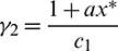and we get

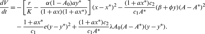
Applying Sylvester criterion, is negative definite if conditions in (17) hold. Hence E* is globally stable under conditions in (17).

3.3 Hopf-Bifurcation and Its Properties

Hopf-bifurcation is a local phenomenon where a system’s stability switches and a periodic solution arises around its equilibrium point by varying a parameter. In system (1), the parameter A0 seems crucial, therefore we analyze the Hopf-bifurcation by taking A0 as bifurcation parameter, then we have some . The necessary and sufficient conditions for occurrence Hopf-bifurcation at are

a)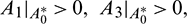    

b)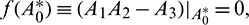    

c) 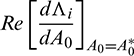    is either positive or negative, where 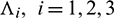are roots of Eq. (14).

From A1A2 − A3 = 0, we get an equation in A0 and assume that it has at least one positive root Then for some there is an interval containing such that and A2 > 0 for Thus, Eq. (14) cannot have any real positive root for

Therefore, at , Eq. (14) becomes

this gives us three roots

where and .

For roots can be taken as

Now, we have to verify the transversality condition. Differentiating Eq. (14) with respect to the bifurcation parameter A0, we obtain

where R = A1A2 − A3 and , i = 1, 2, 3 denote the derivative of Ai with respect to time. Thus

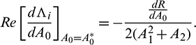
Thus, we can state the following theorem.

Theorem 3.6. The system undergoes Hopf-bifurcation near interior equilibrium E*(x*, A*, y*) under the necessary and sufficient conditions (a), (b) and (c). Critical value of bifurcation parameter A0 is given by the equation

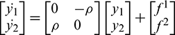
In order to see the stability and direction of Hopf-bifurcation, we use center manifold theorem [34] and some concepts used in [41]. Now, consider the following transformation

Using this transformation, system (1) takes the following form

where X = (x1, x2, x3)T,

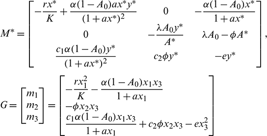
Let v1 and v2 be the eigenvectors corresponding to eigenvalues and of E* at Then v1 and v2 are given by

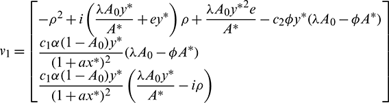
and

Let

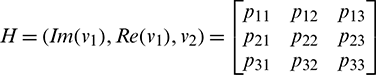
where

Now let X = HY or Y = H−1X, where Y = (y2, y2, y3)T. Using this transformation, system (18) can be written as

where

So, we can write system (19) as

Thus, system (20) takes the following form

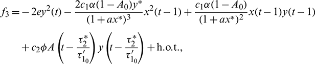
where and g = (f3). The eigenvalues of B and C may have zero real part and negative real parts, respectively. f, g vanish along with their first partial derivative at the origin.

Since the center manifold is tangent to WC (y = 0) we can represent it as a graph

where is defined on some vicinity of the origin [42,43].

We consider the projection of vector field on V = h(U) onto WC:

Now we state the following theorem to approximate the center manifold.

Theorem 3.7. Let be a C1 mapping of a neighborhood of the origin in R2 into R with and If for some as then as where

In order to approximate h(U), we consider

where h.o.t. stands for high order terms. Using (23), we get from (22)

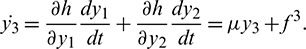
After simplification, we get

where

Equating both the sides of Eq. (24), we get

Using Crammer’s rule,

We can find the behavior of the solution of system (21) from the following theorem.

Theorem 3.8. If the zero solution of (22) is stable (asymptotically stable/unstable), then the zero solution of (21) is also stable (asymptotically stable/unstable).

Now from Eq. (22), we have

where

Let 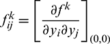and 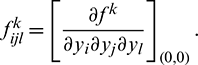Therefore,

We determine the direction and stability of bifurcation periodic orbit of the system (21) by the following formula [44]

In above expression, if then the Hopf-bifurcation is supercritical (subcritical) and bifurcation periodic solution exists for The bifurcating periodic solution is stable (unstable) if

The bifurcating direction of periodic solution of the system (1) is same as the system (21).

3.4 Numerical Simulation

To validate our theoretical findings of model (1), we perform some numerical simulations using MATLAB R2018b. We have chosen the following dataset

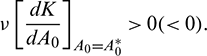
For the above set of parameters, condition for existence of prey free equilibrium (5) and conditions for existence and uniqueness of interior equilibrium (9) and (10) are satisfied. Therefore, the system (1) has five equilibrium points. The behavior of these equilibrium points are given in Tab. 2.

Table 2: Existing equilibria and their stability nature

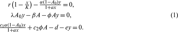
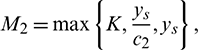
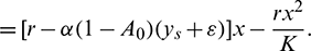
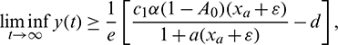
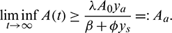
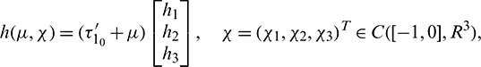
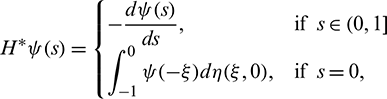
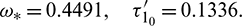
The eigenvalues of the Jacobian matrix at E0 and E1 are (3, −0.32, −0.3) and (−3, −0.32, 0.4113), respectively. Therefore E0 and E1 both are saddle points. Similarly and are also saddle points. Again all the inequalities in (15) are satisfied. So according to Theorem 3.4, the interior equilibrium E* is locally asymptotically stable. The stability of system in the vicinity of the positive equilibrium E* is illustrated by Fig. 2. In Fig. 2a, time evolution of species is shown and it is noted that they converge to their equilibrium levels after some oscillations. In Fig. 2b, phase diagram is drawn in xAy-space which shows the asymptotic stability behavior of positive equilibrium E*.

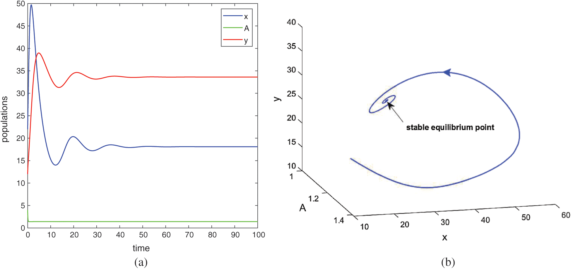
Figure 2: Time series evolution (a) and phase portrait (b) of species for the set of parameters chosen in (25). Positive equilibrium E* is locally asympeoeically stable

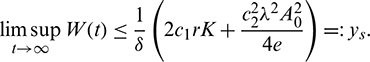
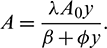
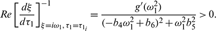
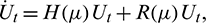
In this study, we found that predators dependency factor A0 on additional food plays an important role in the dynamics of the system. If it is less than a threshold value then it can be the cause of destabilizing the system. The threshold value can be calculated by solving (Theorem 3.6). 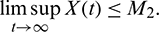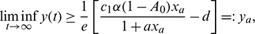By our computer simulation we obtain it as All the conditions of Theorem 3.6 are satisfied, so the system undergoes a Hopf-bifurcation at If we keep the value of parameter A0 below its threshold value, then the system (1) always remains unstable. 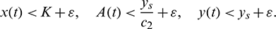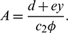The instable behavior of solutions and presence of stable limit cycle at is shown in Fig. 3. In Fig. 4, we draw the bifurcation diagram with respect to parameter A0 for both prey and predator species. From the figure, it is noted that the periodic solution present in the system when and oscillations can be removed from the system by increasing the parameter A0 beyond

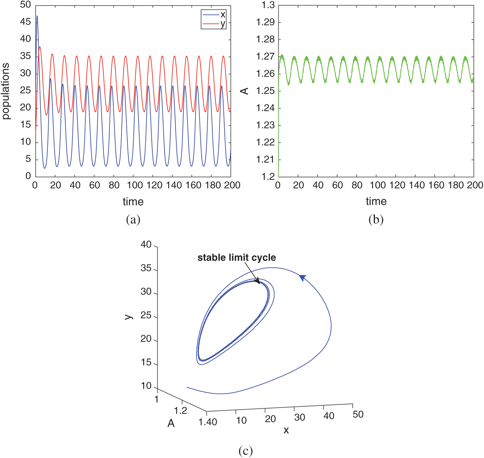
Figure 3: Instable behavior of solutions and existence of stable limit cycle for Rest of the parameters are same as (25)

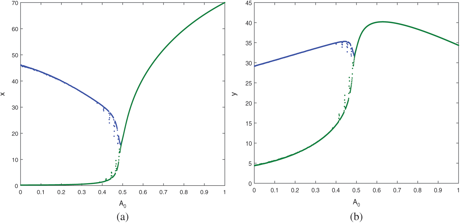
Figure 4: Bifurcation diagram of the prey and predator population with respect to parameter A0

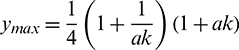
In the model (1), consumption rate of additional food is also a vital parameter. We have noted that if system is stable for parameter then it is stable for all range of parameter But if then system undergoes a Hopf-bifurcation with respect to parameter In Fig. 5, we have shown the bifurcation diagram when A0 = 0.4 and other parameters are same as given in (25). The Hopf-bifurcation point is

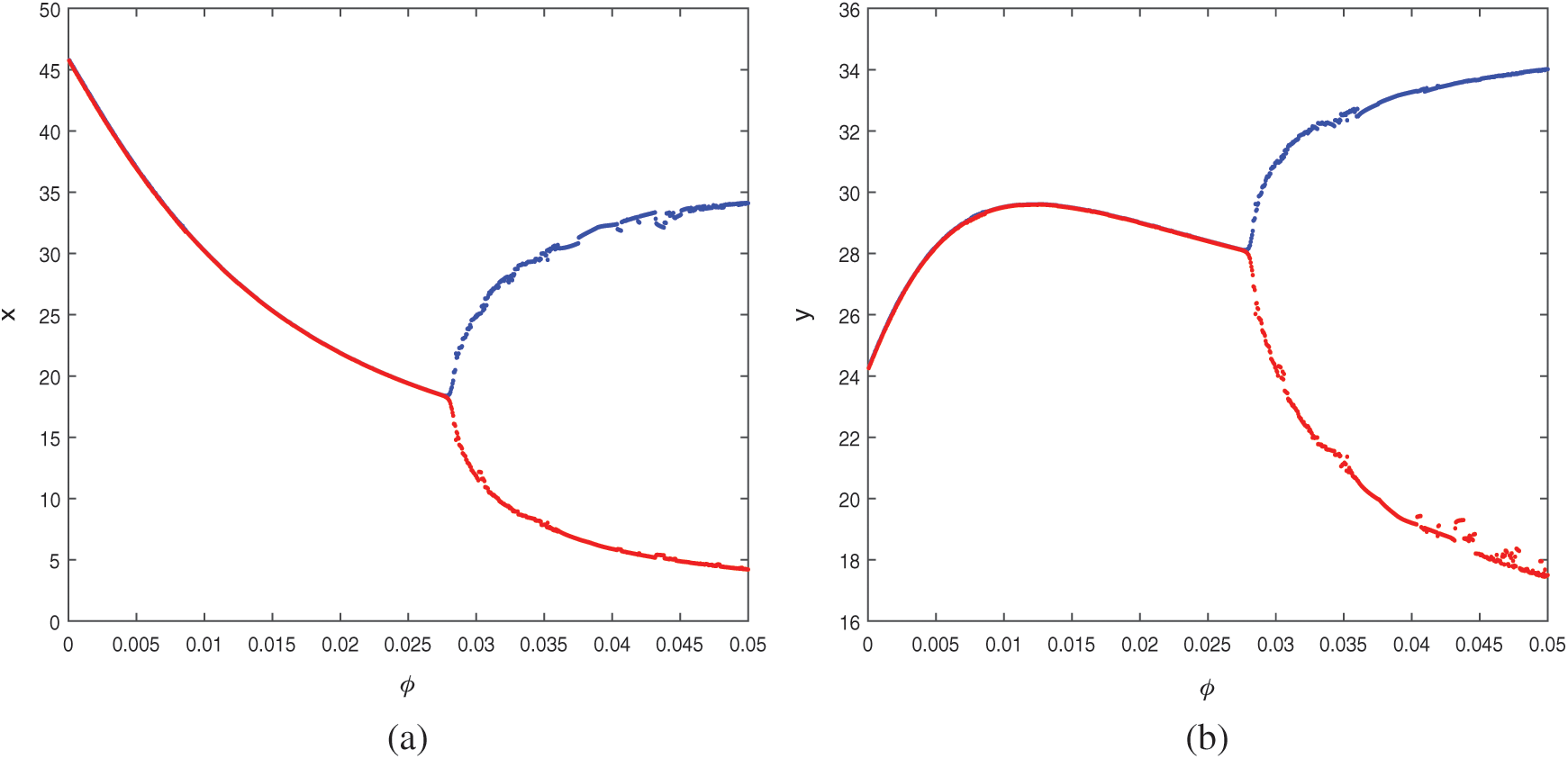
Figure 5: Bifurcation diagram of the prey and predator population with respect to parameter

As the system (1) shows Hopf-bifurcation with respect to parameters A0 and and direction of Hopf-bifurcation is opposite for both the parameters. Therefore, we can divide the -plane into two regions

Region of stability (green) S1 = { system (1) is locally asymptotically stable},

Region of instability (white) S2 = { system (1) is unstable}.

Both the regions are drawn in Fig. 6. The curve which separates both the regions is called Hopf-bifurcation curve.

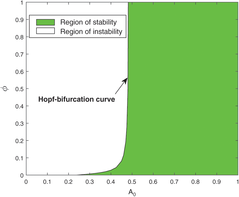
Figure 6: Region of stability and instability for system (1) in -plane

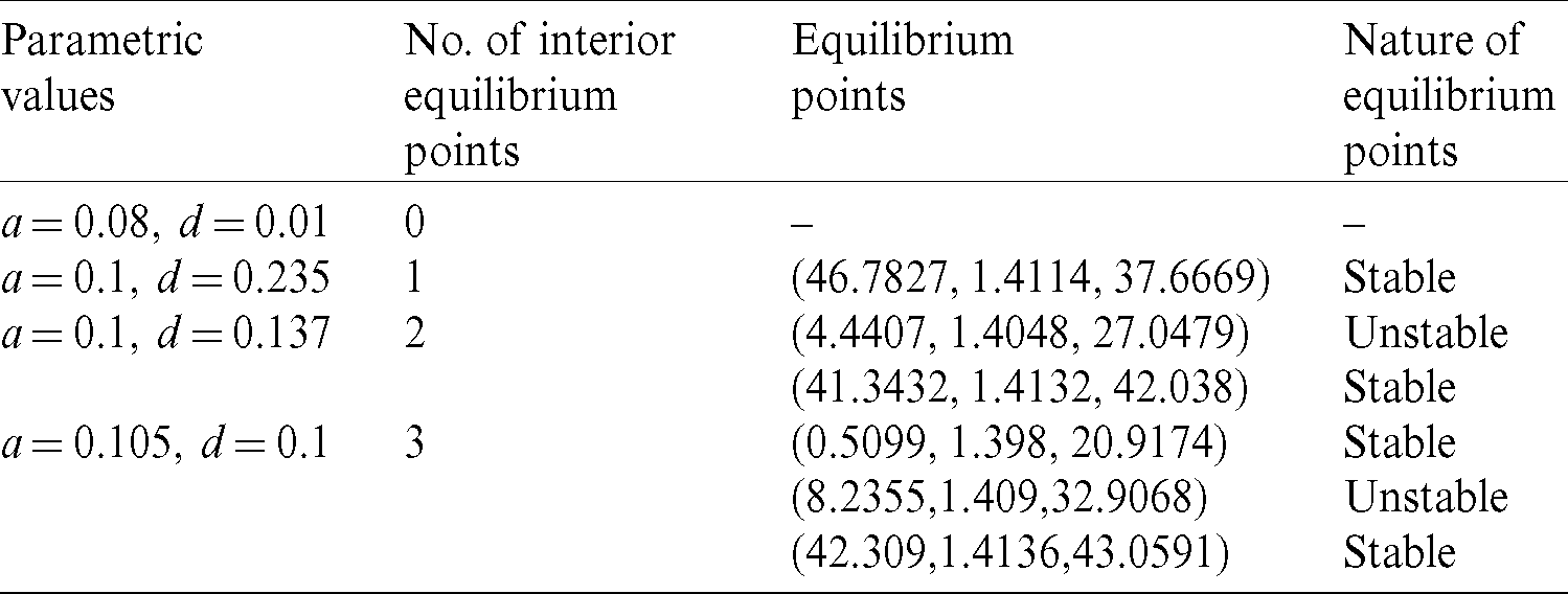
The number of interior equilibrium points depend on the values of parameters. In the table below, we have shown dependence of total number of interior equilibrium on parameters a and d and the nature of their stability. It is observed that when a = 0.105 and d = 0.1 (other parameters are as in (25)), then three interior equilibrium exist for the system (1), and and are locally asymptotically stable and is unstable. Since there are two locally asymptotically stable equilibrium in the system, so it shows bistability. Bistability is a phenomenon where a system converges to two different equilibrium points for the same parametric values based on the variation of the initial conditions. In Fig. 7, we initiated two trajectories from two nearby points and they converse to different interior equilibria. The black dotted curve is separatrix, which divides the xy-plane into two regions in such a way that if a solution is initiated from the left of the separatrix, it converses to and if a solution is initiated from the right of the separatrix, it converses to In other words, left region is region of attraction for and right region is region of attraction for

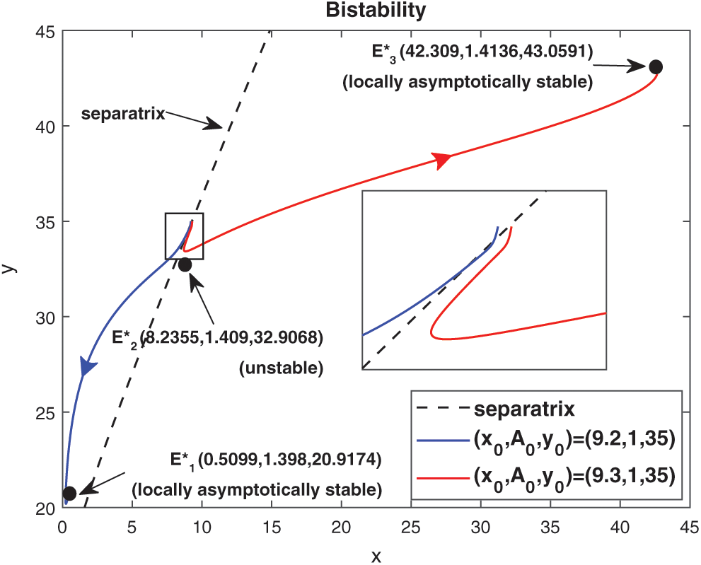
Figure 7: Trajectories initiated from region of attraction of both the locally asymptotically stable equilibrium points, system (1) shows bistability

Remark. For the best representation of bistability phenomenon and separatrix curve, the Fig. 7 is drawn in the xy-plane. But initial conditions and interior equilibrium points are written as they are.

4  Analysis of Delayed Model

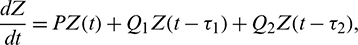
In this section, we discuss the local stability and Hopf-bifurcation phenomenon for the delayed system (2). The introduction of time delay does not affects the equilibria of the system. So, all the equilibria remain same as the non-delayed system (1). To see the effect of delay on the dynamical behavior of the interior equilibrium E*, we rewrite the delayed system (2) as

where

Now we linearize the system (26) by using the following transformations:

where , and are small perturbations around x*, A* and y*, respectively. Then the linearized system of (26) about the interior equilibrium E* is given by

where

Thus, the Jacobian matrix of the system (2) at E* is given by

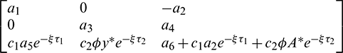
where

The characteristic equation corresponding to the above Jacobian matrix is

where

Remark. When , then the characteristic Eq. (27) is same as the characteristic Eq. (14) for non-delayed system.

Case (1): , . Then Eq. (27) becomes

where

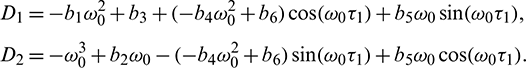
For the delayed system (2), the positive equilibrium is locally asymptotically stable if and only if all the roots of the Eq. (28) have negative real parts. For switching of the stability, the root of the Eq. (28) must cross the imaginary axis. Therefore let be a root of Eq. (28), then it follows that

From the above set of equations, we can obtain

where

If we put , then Eq. (30) becomes

Theorem 4.1. If Eq. (31) has no positive root, then there is no change in the stability behavior of E* for all .

Corollary. If inequalities in (15) hold and Eq. (31) has no positive root, then E* is locally asymptotically stable for all .

Corollary. If inequalities in (15) do not hold and Eq. (31) has no positive root, then E* is unstable for all

Now let inequalities in (15) hold and Eq. (31) has at least one positive root, say . Substituting into Eq. (29), we obtain

.

Let 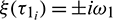be the root of Eq. (28), a little calculation yields

But sign of 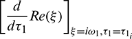is same as the sign of .

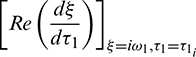Hence, the transversality condition can be obtained under (H1)

Thus, we can state the following theorem.

Theorem 4.2. For system (2), with and assuming that (H1) holds, there exists a positive number such that the equilibrium E* is locally asymptotically stable when and unstable when . Furthermore system (2) undergoes a Hopf-bifurcation at E* when

Case (2): , . Then Eq. (27) becomes

where

Under an analysis similar to Case (1), one can easily deduce the following theorem.

Theorem 4.3. For , the interior equilibrium point is locally asymptotically stable for unstable for and it undergoes Hopf-bifurcation at given by

where is root of characteristic Eq. (33).

Case (3): is fixed in the interval and assuming as a variable parameter.

We consider Eq. (27) with as fixed in its stable interval and as a variable. Let be a root of characteristic Eq. (27). Then separating real and imaginary parts, we obtain

Squaring and then adding (34) and (35) to eliminate , we obtain

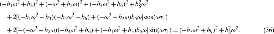
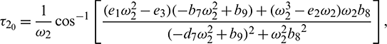
Eq. (36) is a transcendental equation in complex form. So, it is not easy to predict the nature of roots. Without going detailed analysis with (36), it is assumed that there exist at least one positive root . Eqs. (34) and (35) can be re-written as

where

Eqs. (37) and (38) lead to

Now, to verify the transversality condition of Hopf-bifurcation, differentiating equation (34) and (35) with respect to and substitute , we obtain

where

Solving Eq. (40) for , it is obtained

Theorem 4.4. For system (2), with and assuming that (H2) holds, there exists a positive number such that E* is locally asymptotically stable when and unstable when . Furthermore, system (2) undergoes a Hopf-bifurcation at E* where

Case (4): is fixed in the interval and assuming as a variable parameter Under an analysis similar to Case (3), one can easily prove the following theorem.

Theorem 4.5. For the interior equilibrium point is locally asymptotically stable for and it undergoes Hopf-bifurcation at , given by

where

and is characteristic root of Eq. (27).

5  Direction and Stability of Hopf-Bifurcation

Now with the help of center manifold theory and normal form concept (see [34] for details), we shall study direction and stability of the bifurcated periodic solutions at

Without loss of generality, we assume that , where Let

and still denote x1(t), A1(t), y1(t) by x(t), A(t), y(t). Let , so that Hopf-bifurcation occurs at . We normalize the delay with scaling , then system (2) can be re-written as

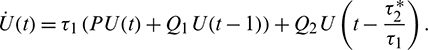
where U(t) = (x(t), A(t), y(t))T,

The nonlinear term f1, f2 and f2 are given by

The linearization of Eq. (41) around the origin is given by

For , define

By the Riesz representation theorem, there exists a matrix , whose element are of bounded variation function such that

In fact, we can obtain

Then Eq. (42) is satisfied.

For define the operator as

and

where

Then system (2) is equivalent to the following operator equation

where 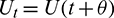for .

For 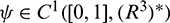, define

and a bilinear form

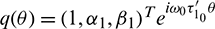
where , H = H(0) and H* are adjoint operators. From the discussion in previous section, we know that are the eigenvalues of H(0) and therefore they are also eigenvalues of H*. It is not difficult to verify that the vectors and are the eigenvectors of H(0) and H* corresponding to the eigenvalue and respectively, where

Following the algorithms explained in Hassard et al. [34] and using a computation process similar to that in Song et al. [26], which is used to obtain the properties of Hopf-bifurcation, we obtain

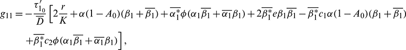
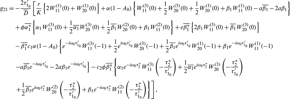
where

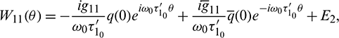
and 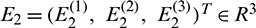are constant vectors, computed as:

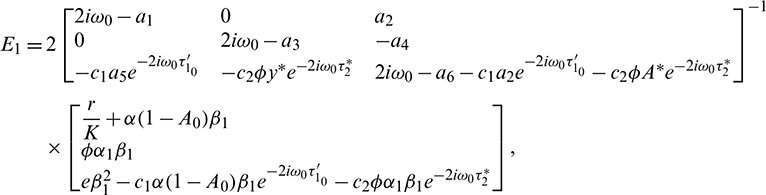
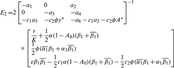
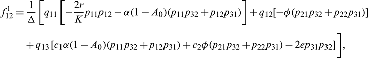
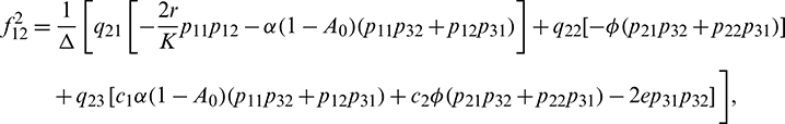
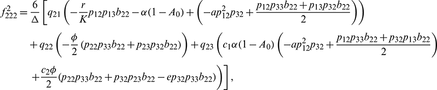
Consequently, gij can be expressed by the parameters and delays and . Thus, these standard results can be computed as:

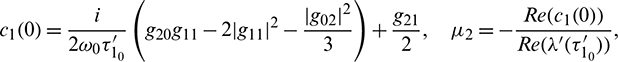
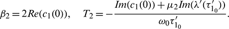
These expressions give a description of the bifurcating periodic solution in the center manifold of system (2) at critical values which can be stated in the form of following theorem:

Theorem 5.1

•     determines the direction of Hopf-bifurcation. If 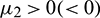then the Hopf-bifurcation is supercritical (subcritical).

•     determines the stability of bifurcated periodic solution. If then the bifurcated periodic solutions are unstable (stable).

•    T2 determines the period of bifurcating periodic solution. The period increases (decreases) if T2 > 0(< 0).

Remark. When and or and , then under an analysis similar to Section 5, the corresponding values of , and T2 can be computed. Depending upon the sign of , and T2, the corresponding results can also be deduced.

6  Numerical Simulation of Delayed Model

In order to validate our theoretical findings, obtained in previous sections, we perform some simulations by taking the same values of parameters in (25). We consider all four cases on delay parameters and .

Case (I): When and , then we see that condition (H1) holds. Since the transversality condition is satisfied, therefore Hopf-bifurcation occurs in the system. To evaluate the critical value of delay parameter, taking i = 0 in Eqs. (31) and (32), we obtain

Thus, the positive equilibrium is locally asymptotically stable for , which is shown in Fig. 8. When , system undergoes a Hopf-bifurcation and periodic solution occurs around E*. The time series analysis and periodic solution have been shown in Fig. 9. If we starts a trajectory from an initial point then it approaches to the periodic solution (Fig. 9). This shows that the periodic solution is stable. In Fig. 10, we made the bifurcation diagram for both the populations. The blue (red) curve represents the maximum (minimum) values of population at sufficiently large time. It is easy to see that Hopf-bifurcation occurs at .

Figure 8: Time series evolution and phase portrait of species for the set of parameters in (25) and 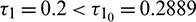when . System is locally asymptotically stable around the positive equilibrium E*

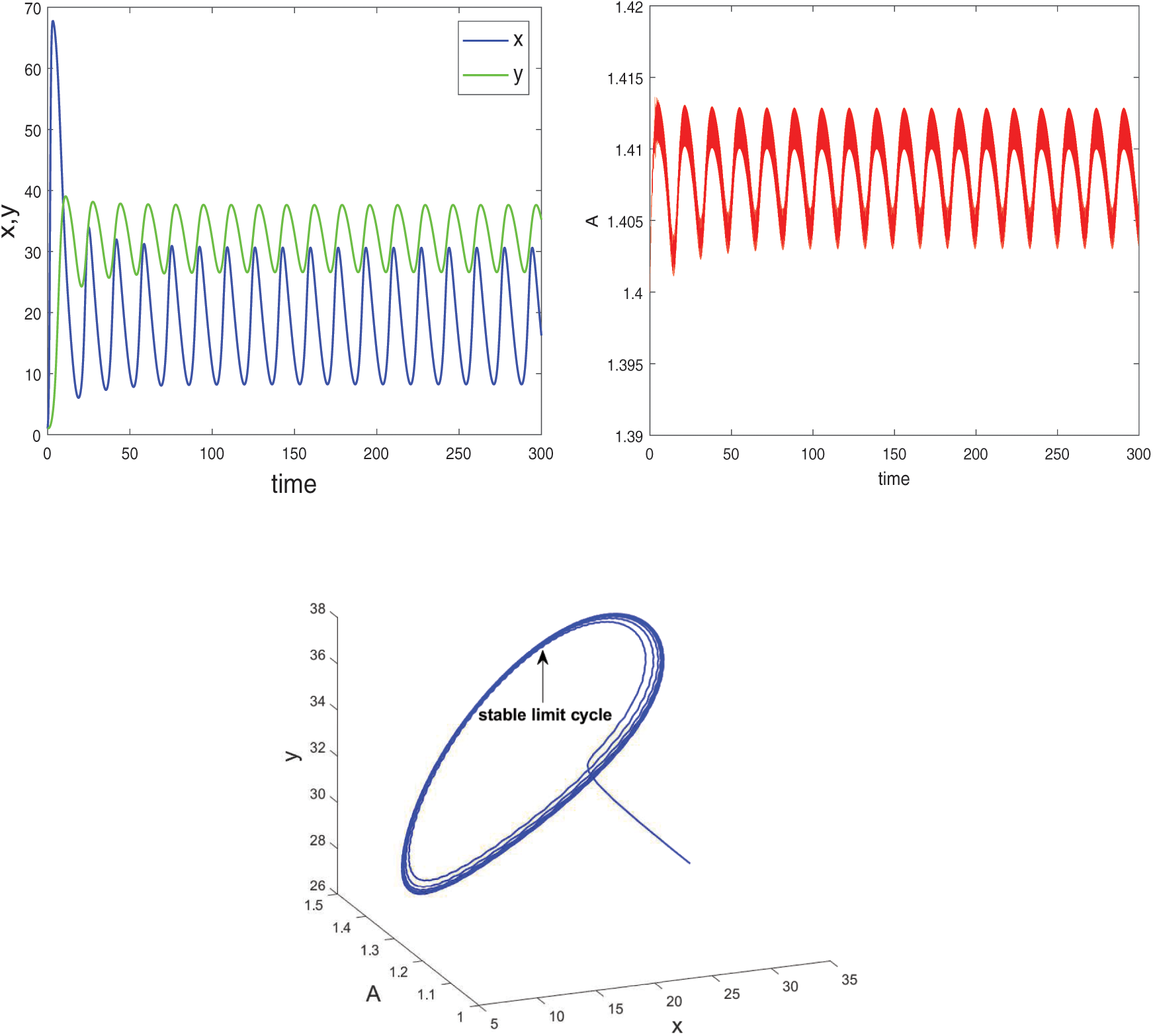
Figure 9: System (2) is unstable when and Hopf-bifurcation occurs and stable limit cycle arises in the system

Figure 10: Bifurcation diagram of the prey and predator population with respect to delay parameter when

Case (II): When and . In this case, the transversality condition is satisfied, so the system will show Hopf-bifurcation at a critical value of delay parameter By some computation, we obtain

Therefore, according to our theoretical analysis, the system (2) is locally asymptotically stable for . In Fig. 11, we draw the time series of both the species for . From the figure, it can be seen that system is stable around the positive equilibrium E*. At , the system goes through a Hopf-bifurcation and for , system becomes unstable and limit cycle produces. This behavior is depicted in Fig. 12. Again bifurcation diagram with respect to delay for both the species is drawn in Fig. 13, which helps us to understand the Hopf-bifurcation phenomenon in the system.

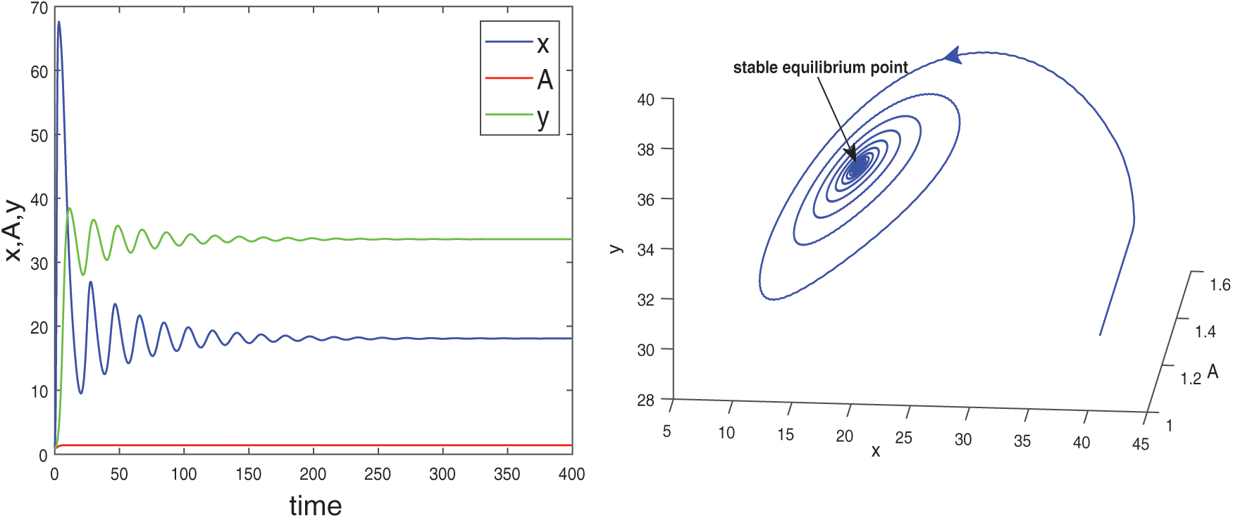
Figure 11: Stable time series solutions and phase diagram of system (2) for 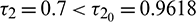and . Other parameters are same as in (25)

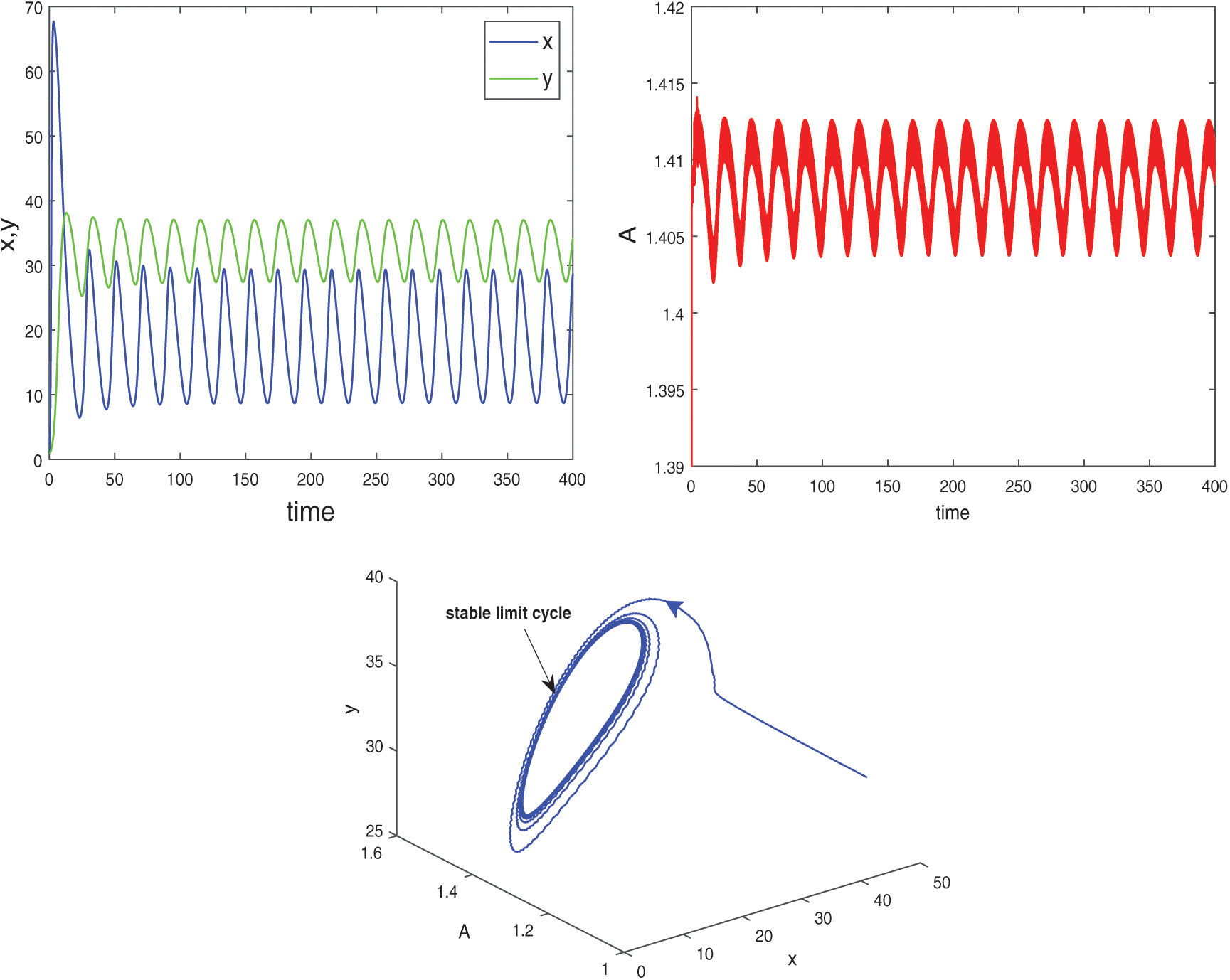
Figure 12: Instable behavior and existence of periodic solutions of system (2) around the positive equilibrium E* at 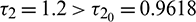and

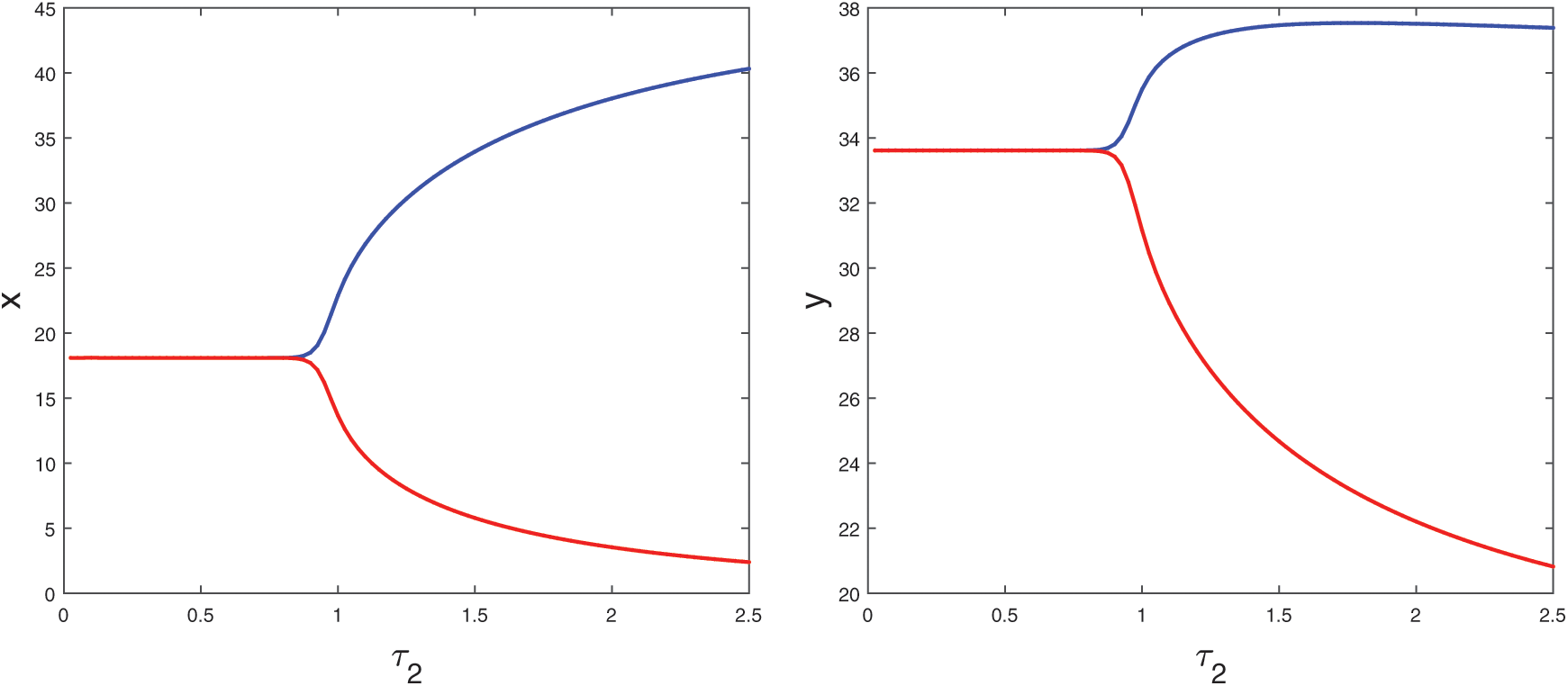
Figure 13: Bifurcation diagram of the prey and predator population with respect to delay parameter and

Case (III): When (fixed in the interval ) and as a parameter, then we observe that the condition (H2) holds true. Therefore according to Theorem 4.4 system (2) undergoes a Hopf-bifurcation. Eqs. (36) and (39) give us the values of and as

Thus the equilibrium point E* is locally asymptotically stable for 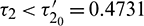which is shown in Fig. 14 and unstable for (Fig. 15). When , system undergoes a Hopf-bifurcation around E* and periodic solution arises in the system. Bifurcation diagram is also presented in Fig. 16 with respect to for both the species when (fixed).

Figure 14: E* is locally asymptotically stable when is fixed in its stable range and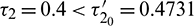

Figure 15: E* is unstable when is fixed in its range of stability and 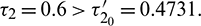Time series solution of species and existence limit cycle

Figure 16: Bifurcation diagram of the prey and predator species with respect to parameter when is fixed in its range of stability

Case (IV): When (fixed in the interval ) and as a parameter, then our computer simulation yields

For , the system is locally asymptotically stable (Fig. 17). But for , the system becomes unstable (Fig. 18). Thus the model is stable for . As passes through , it loses the stability and a Hopf-bifurcation occurs in the system. Fig. 18 shows the existence of periodic solution (closed trajectory). The trajectory started from an initial point, approaches to the closed trajectory. This shows that the closed trajectory is stable. In Fig. 19, we present the bifurcation diagram of both the species with respect to when (fixed).

Figure 17: E* is locally asymptotically stable when is fixed in its stable range and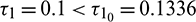

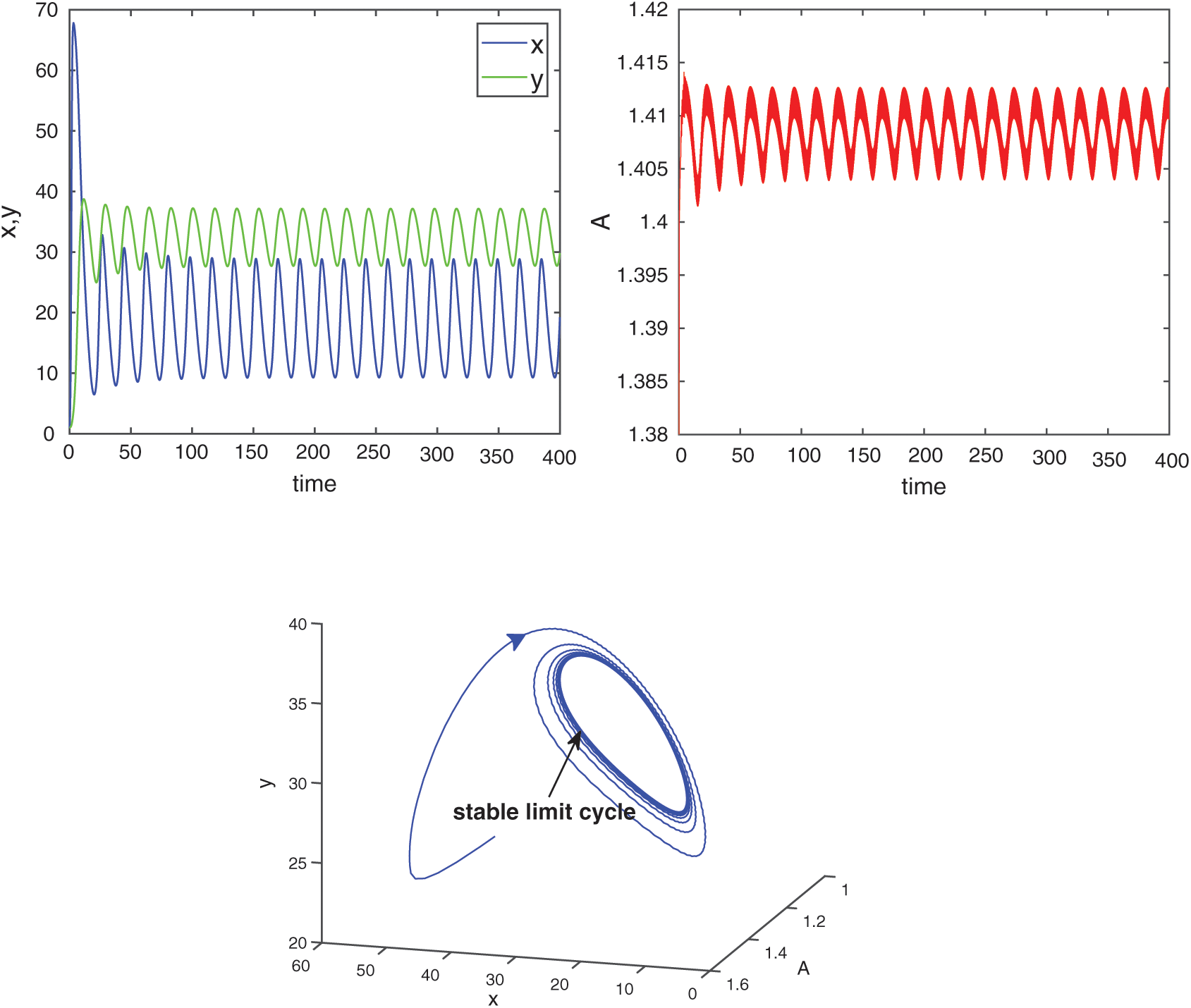
Figure 18: E* is unstable when is fixed in its stable range and . Time series solution of species and existence limit cycle

Figure 19: Bifurcation diagram of the prey and predator species with respect to parameter when is fixed in its stable range

As the system (2) shows Hopf-bifurcation with respect to both the delay parameters and . Therefore, we can bisect the –-plane into two regions, which are separated by Hopf-bifurcation curve.

Both the regions are drown in Fig. 20.

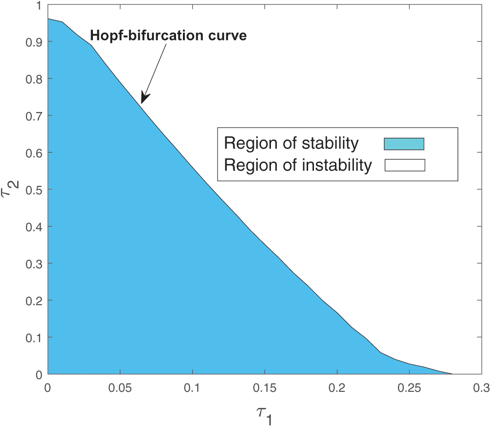
Figure 20: Region of stability and instability for system (2) in -plane

7  Conclusion

In this study, we have considered a habitat where two biological populations, prey population x and predator population y are surviving and interacting with each other. It is assumed that prey population follows logistic growth in the absence of predator and in the presence of predator, the interaction between them follows Holling type II functional response. We have shown the positivity, boundedness and persistence of the system, which implies that the proposed model is ecologically wellposed. We have defined a parameter A0 ( which denotes the dependency of predators on supplied additional food. Our system has four kinds of equilibria, trivial equilibrium E0(0, 0, 0), axial equilibrium E1(K, 0, 0), two prey free equilibria and under condition (5) and unique positive equilibrium E* under conditions (9) and (10). Local and global stability of the positive equilibrium are shown under several conditions which are dependent upon the parameter A0. The parameter A0 is crucial, so we have studied its effect via Hopf-bifurcation analysis which is also condescend by the numerical illustration. For a chosen set of parameters we calculated the threshold value of parameter A0, that is A0 = 0.482, where Hopf-bifurcation occurs and system stabilizes. It is also observed that after stabilization of system if predators are more dependent on additional food then prey population increase whereas predators remain in their range. We also have studied the Hopf-bifurcation with respect to consumption rate of additional food . Threshold value of is obtained as 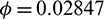. In Tab. 3, we have shown the different number of positive equilibrium points by varying the parametric values, when a = 0.105 and d = 0.1 (other parameters are same as in (25)) then our system has two stable equilibrium together, therefore system shows the phenomenon of bistability, which is depicted in Fig. 7.

Table 3: Dependence of total number of interior equilibria and their stability on parameters a and d. Rest of the parameters are same as in (25)

Models with delay show comparatively more realistic dynamics than non delayed models. When a predator consumes a prey individual, then its effect does not come immediately, it takes some time i.e., time lag for gestation. Again, predators also take some time to consume and digest the supplied additional food to them. Therefore, to make our model ecologically more realistic, we incorporated two delays; one for gestation delay and other for consuming and digesting the supplied additional food.

For the delayed model, we have analyzed Hopf-bifurcation via local stability taking delay as a bifurcation parameter. We investigated the Hopf-bifurcation phenomenon for all combinations of both delays. We obtained the sufficient conditions for the stability of the positive equilibrium point and existence of Hopf-bifurcation for Case(1): , , Case(2): , , Case(3): is fixed in the interval and as a variable parameter, Case(4): is fixed in the interval and as a variable parameter. Our system undergoes Hopf-bifurcation in the vicinity of the interior equilibrium point with respect to both the delay parameters when they cross their critical values. The qualitative properties of Hopf-bifurcation are studied by using the Normal form theory and the formulae given in Hassard et al. [34].

We have performed some numerical simulations to illustrate our theoretical results. For a biologically feasible set of parameters, the system is stable initially, then we introduce delay and system remains stable till its critical value. If we increase the delay parameter over the critical value, then system goes through Hopf-bifurcation and becomes unstable. Bifurcation diagrams (Figs. 10, 13, 16, 19) with respect to different delays depict the dynamical behavior of the system.

Our study is important to conserve the prey population through providing additional food to predators and to establish their balance. Here we have also shown the significance of delay parameters. We hope that this study will help to perceive the dynamics of an ecological system with additional food and two discrete delays.

Acknowledgement: The author (Ankit Kumar) acknowledges the Junior Research Fellowship received from University Grant Commission, New Delhi, India.

Funding Statement: The authors received no specific funding for this study.

Conflicts of Interest: The authors declare that they have no conflicts of interest to report regarding the present study.

References

 1.  Lotka, A. J. (1925). Elements of physical biology. Baltimore, New York: Williams and Wilkins. [Google Scholar]

 2.  Volterra, V. (1927). Variazioni e fluttuazioni del numero d’individui in specie animali conviventi. Venezia, C. Ferrari. [Google Scholar]

 3.  Ma, Z., Wang, S. (2018). A delay-induced predator-prey model with Holling type functional response and habitat complexity. Nonlinear Dynamics, 93(3), 1519–1544. DOI 10.1007/s11071-018-4274-2. [Google Scholar] [CrossRef]

 4.  Dubey, B., Kumar, A., Maiti, A. P. (2019). Global stability and Hopf-bifurcation of prey–predator system with two discrete delays including habitat complexity and prey refuge. Communications in Nonlinear Science and Numerical Simulation, 67, 528–554. DOI 10.1016/j.cnsns.2018.07.019. [Google Scholar] [CrossRef]

 5.  Holling, C. S. (1959). The components of predation as revealed by a study of small-mammal predation of the European pine sawfly. The Canadian Entomologist, 91(5), 293–320. DOI 10.4039/Ent91293-5. [Google Scholar] [CrossRef]

 6.  Crowley, P. H., Martin, E. K. (1989). Functional responses and interference within and between year classes of a dragonfly population. Journal of the North American Benthological Society, 8(3), 211–221. DOI 10.2307/1467324. [Google Scholar] [CrossRef]

 7.  Wang, W., Chen, L. (1997). A predator–prey system with stage–structure for predator. Computers & Mathematics with Applications, 33(8), 83–91. DOI 10.1016/S0898-1221(97)00056-4. [Google Scholar] [CrossRef]

 8.  Faria, T. (2001). Stability and bifurcation for a delayed predator–prey model and the effect of diffusion. Journal of Mathematical Analysis and Applications, 254(2), 433–463. DOI 10.1006/jmaa.2000.7182. [Google Scholar] [CrossRef]

 9.  Prasad, B. S. R. V., Banerjee, M., Srinivasu, P. D. N. (2013). Dynamics of additional food provided predator–prey system with mutually interfering predators. Mathematical Biosciences, 246(1), 176–190. DOI 10.1016/j.mbs.2013.08.013. [Google Scholar] [CrossRef]

10. Li, H., Meng, G., She, Z. (2016). Stability and Hopf bifurcation of a delayed density–dependent predator–prey system with Beddington–DeAngelis functional response. International Journal of Bifurcation and Chaos, 26(10), 1650165. DOI 10.1142/S0218127416501650. [Google Scholar] [CrossRef]

11. Wang, X., Zanette, L., Zou, X. (2016). Modelling the fear effect in predator–prey interactions. Journal of Mathematical Biology, 73(5), 1179–1204. DOI 10.1007/s00285-016-0989-1. [Google Scholar] [CrossRef]

12. Li, H. L., Zhang, L., Hu, C., Jiang, Y. L., Teng, Z. (2017). Dynamical analysis of a fractional-order predator–prey model incorporating a prey refuge. Journal of Applied Mathematics and Computing, 54(1–2), 435–449. DOI 10.1007/s12190-016-1017-8. [Google Scholar] [CrossRef]

13. Dong, Q., Ma, W., Sun, M. (2013). The asymptotic behavior of a chemostat model with Crowley–Martin type functional response and time delays. Journal of Mathematical Chemistry, 51(5), 1231–1248. DOI 10.1007/s10910-012-0138-z. [Google Scholar] [CrossRef]

14. Maiti, A. P., Dubey, B., Tushar, J. (2017). A delayed prey–predator model with Crowley–Martin-type functional response including prey refuge. Mathematical Methods in the Applied Sciences, 40(16), 5792–5809. DOI 10.1002/mma.4429. [Google Scholar] [CrossRef]

15. Srinivasu, P. D. N., Prasad, B. S. R. V., Venkatesulu, M. (2007). Biological control through provision of additional food to predators: A theoretical study. Theoretical Population Biology, 72(1), 111–120. [Google Scholar]

16. Ddumba, H., Mugisha, J. Y. T., Gonsalves, J. W., Kerley, G. I. H. (2013). Periodicity and limit cycle perturbation analysis of a predator–prey model with interspecific species’ interference, predator additional food and dispersal. Applied Mathematics and Computation, 219(15), 8338–8357. DOI 10.1016/j.amc.2012.11.063. [Google Scholar] [CrossRef]

17. Sahoo, P., Poria, S. (2014). The chaos and control of a food chain model supplying additional food to top-predator. Chaos, Solitons & Fractals, 58, 52–64. [Google Scholar]

18. Kumar, D., Chakrabarty, S. P. (2015). A comparative study of bioeconomic ratio-dependent predator-prey model with and without additional food to predators. Nonlinear Dynamics, 80(1–2), 23–38. [Google Scholar]

19. Sen, M., Srinivasu, P. D. N., Banerjee, M. (2015). Global dynamics of an additional food provided predator-prey system with constant harvest in predators. Applied Mathematics and Computation, 250, 193–211. [Google Scholar]

20. Ghosh, J., Sahoo, B., Poris, S. (2017). Prey-predator dynamics with prey refuge providing additional food to predator. Chaos, Solitons & Fractals, 96, 110–119. [Google Scholar]

21. Sahoo, B. (2015). Role of additional food in eco-epidemiological system with disease in the prey. Applied Mathematics and Computation, 259, 61–79. DOI 10.1016/j.amc.2015.02.038. [Google Scholar] [CrossRef]

22. Rani, R., Gakkhar, S. (2019). The impact of provision of additional food to predator in predator–prey model with combined harvesting in the presence of toxicity. Journal of Applied Mathematics and Computing, 60(1–2), 673–701. DOI 10.1007/s12190-018-01232-z. [Google Scholar] [CrossRef]

23. Bairagi, N., Jana, D. (2011). On the stability and Hopf bifurcation of a delay-induced predator–prey system with habitat complexity. Applied Mathematical Modelling, 35(7), 3255–3267. DOI 10.1016/j.apm.2011.01.025. [Google Scholar] [CrossRef]

24. Tripathi, J. P., Abbas, S., Thakur, M. (2015). A density dependent delayed predator–prey model with Beddington–DeAngelis type function response incorporating a prey refuge. Communications in Nonlinear Science and Numerical Simulation, 22(1–3), 427–450. DOI 10.1016/j.cnsns.2014.08.018. [Google Scholar] [CrossRef]

25. Gourley, S. A., Kuang, Y. (2004). A stage structured predator–prey model and its dependence on maturation delay and death rate. Journal of Mathematical Biology, 49(2), 188–200. DOI 10.1007/s00285-004-0278-2. [Google Scholar] [CrossRef]

26. Song, Y., Wei, J. (2004). Bifurcation analysis for Chen’s system with delayed feedback and its application to control of chaos. Chaos, Solitons & Fractals, 22(1), 75–91. DOI 10.1016/j.chaos.2003.12.075. [Google Scholar] [CrossRef]

27. Qu, Y., Wei, J. (2007). Bifurcation analysis in a time-delay model for prey–predator growth with stage–structure. Nonlinear Dynamics, 49(1–2), 285–294. DOI 10.1007/s11071-006-9133-x. [Google Scholar] [CrossRef]

28. Misra, A. K., Dubey, B. (2010). A ratio-dependent predator–prey model with delay and harvesting. Journal of Biological Systems, 18(2), 437–453. DOI 10.1142/S021833901000341X. [Google Scholar] [CrossRef]

29. Chakraborty, K., Jana, S., Kar, T. K. (2012). Effort dynamics of a delay-induced preypredator system with reserve. Nonlinear Dynamics, 70(3), 1805–1829. [Google Scholar]

30. Gakkhar, S., Singh, A. (2012). Complex dynamics in a prey predator system with multiple delays. Communications in Nonlinear Science and Numerical Simulation, 17(2), 914–929. DOI 10.1016/j.cnsns.2011.05.047. [Google Scholar] [CrossRef]

31. Jana, S., Chakraborty, M., Chakraborty, K., Kar, T. K. (2012). Global stability and bifurcation of time delayed prey–predator system incorporating prey refuge. Mathematics and Computers in Simulation, 85, 57–77. DOI 10.1016/j.matcom.2012.10.003. [Google Scholar] [CrossRef]

32. Misra, A. K., Lata, K. (2013). Modeling the effect of time delay on the conservation of forestry biomass. Chaos, Solitons & Fractals, 46, 1–11. DOI 10.1016/j.chaos.2012.10.002. [Google Scholar] [CrossRef]

33. Liu, Y., Zhang, X., Zhou, T. (2014). Multiple periodic solutions of a delayed predatorprey model with non-monotonic functional response and stage structure. Journal of Biological Dynamics, 8(1), 145–160. [Google Scholar]

34. Hassard, B. D., Kazarinoff, N. D., Wan, Y. H., Wan, Y. W. (1981). (Theory and applications of Hopf bifurcation. vol. 41. London, UK: CUP Archive. [Google Scholar]

35. Sahoo, B., Poria, S. (2015). Effects of additional food in a delayed predator–prey model. Mathematical Biosciences, 261, 62–73. DOI 10.1016/j.mbs.2014.12.002. [Google Scholar] [CrossRef]

36. Mondal, S., Maiti, A., Samanta, G. P. (2019). Effects of fear and additional food in a delayed predator–prey model. Biophysical Reviews and Letters, 13(4), 157–177. DOI 10.1142/S1793048018500091. [Google Scholar] [CrossRef]

37. Li, K., Wei, J. (2009). Stability and Hopf bifurcation analysis of a prey–predator system with two delays. Chaos, Solitons & Fractals, 42(5), 2606–2613. DOI 10.1016/j.chaos.2009.04.001. [Google Scholar] [CrossRef]

38. Xu, C., Tang, X., Liao, M., He, X. (2011). Bifurcation analysis in a delayed Lokta–Volterra predator–prey model with two delays. Nonlinear Dynamics, 66(1–2), 169–183. DOI 10.1007/s11071-010-9919-8. [Google Scholar] [CrossRef]

39. Xu, C., Li, P. (2012). Dynamical analysis in a delayed predator–prey model with two delays. Discrete Dynamics in Nature and Society, 2012(1), 1–22. DOI 10.1155/2012/652947. [Google Scholar] [CrossRef]

40. Kundu, S., Maitra, S. (2018). Dynamical behaviour of a delayed three species predator–prey model with cooperation among the prey species. Nonlinear Dynamics, 92(2), 627–643. DOI 10.1007/s11071-018-4079-3. [Google Scholar] [CrossRef]

41. Misra, A. K., Verma, M. (2013). A mathematical model to study the dynamics of carbon dioxide gas in the atmosphere. Applied Mathematics and Computation, 219(16), 8595–8609. DOI 10.1016/j.amc.2013.02.058. [Google Scholar] [CrossRef]

42. Carr, J. (2012). Applications of centre manifold theory, vol. 35. Berlin, Germany: Springer Science & Business Media. [Google Scholar]

43. Kuznetsov, Y. A. (2013). (Elements of applied bifurcation theory. vol. 112. Berlin, Germany: Springer Science & Business Media. [Google Scholar]

44. Lin, Y., Zeng, X., Jing, Z. (1996). Dynamical behaviors for a three-dimensional differential equation in chemical system. Acta Mathematicae Applicatae Sinica, 12(2), 144–154. DOI 10.1007/BF02007734. [Google Scholar] [CrossRef]

This work is licensed under a Creative Commons Attribution 4.0 International License, which permits unrestricted use, distribution, and reproduction in any medium, provided the original work is properly cited.