Computer Modeling in Engineering & Sciences

DOI: 10.32604/cmes.2021.011954

ARTICLE

An Uncertainty Analysis Method for Artillery Dynamics with Hybrid Stochastic and Interval Parameters

Liqun Wang1, Zengtao Chen2 and Guolai Yang1,*

1School of Mechanical Engineering, Nanjing University of Science & Technology, Nanjing, 210094, China
2Department of Mechanical Engineering, University of Alberta, Edmonton, T6G 1H9, Canada
*Corresponding Author: Guolai Yang. Email: yangglnjust@gmail.com
Received: 07 June 2020; Accepted: 14 September 2020

1  Introduction

In practical dynamic systems, a variety of uncertainties associated with material properties, environmental factors, external loads, dimensional tolerances, and boundary conditions are ubiquitous. These uncertainties will inevitably affect the final system performances, and small variations associated with uncertainties might result in significant changes in the dynamic responses. The traditional way to investigate the dynamic response problems with uncertainty parameters is the probabilistic method, in which the uncertainty parameters are described as stochastic variables or processes with precise probability distributions. Among these probabilistic methods, Monte Carlo simulation (MCS) [1–3] is considered to be the most accurate and most versatile. Despite the simplicity, it suffers from the considerable computational burden, thus it is usually used to generate the reference solutions. To circumvent this drawback, the stochastic perturbation method [4–6] using first-order or high-order Taylor series expansion was incorporated into MCS to investigate the dynamic response problems. However, it is precise only for the small uncertainty level problems. Wan et al. [7] and Lu et al. [8] presented a general framework for analytical uncertainty quantification of model outputs using a Gaussian process metamodel, where the inputs are characterized as normal and/or uniform random variables, and characterized the uncertainty of modal frequencies of bridge systems. Lu et al. [9] employed modal decomposition together with a low-dimensional representation method to address the curse of dimensionality of frequency response functions output, subsequently provided a fast vector-output approximation of the random modal parameters through multi-output Gaussian process metamodel. Moreover, the spectral stochastic method [10–12] is also an efficient alternative for stochastic problems, of which the polynomial chaos expansion (PCE) method [13–15] has drawn much attention due to its strong power in functional representations of stochastic parameters. PCE has achieved significant successes in dealing with structural dynamic responses. Xiu et al. [13] presented the method for solving stochastic differential equations based on the Galerkin projections and extensions of Wiener’s polynomial chaos. Sandu et al. [16] Saha et al. [17] applied the generalized polynomial chaos to model the complex, nonlinear, multibody dynamic systems with stochastic uncertainty. Saha et al. [18] applied the generalized PCE to stochastic, dynamic response analysis of the base-isolated liquid storage tanks. Wan et al. [19] presented an efficient approach based on arbitrary polynomial chaos expansion for analytical, unified implementation of uncertainty quantification and global sensitivity analysis in structural dynamics. For the aforementioned probabilistic methods, determining precise probability distribution is required, which usually needs complete stochastic information or experimental data. Unfortunately, the objective information is usually insufficient and expensive to obtain in practical engineering problems. In this context, multiple types of non-probabilistic models, such as fuzzy model and interval model, have been used to quantify the uncertainty.

Interval methods depict uncertainty through the upper and lower bounds of uncertain-but-bounded parameters rather than other stochastic information, therefore, they are considered to be a powerful supplement to the classical probabilistic approaches and have been perfectly applied in dynamic structural response analysis. The interval arithmetic operation [20,21] was the first used for dynamic response analysis. We can obtain the approximate response bounds effectively through the specific interval operators. However, its inherent deficiency is the large overestimation of range enclosure namely wrapping effect [22,23], which becomes more obvious and severe in the multidimensional and non-monotonic problems. To this end, some other interval-based, dynamic response analysis methods, such as the Taylor model method [24,25], interval vertex method [26], and the heuristic optimization method [27], have been developed. Based on the first-order or second-order Taylor series expansion, Qiu et al. [28,29], Zhang et al. [30], and Han et al. [31] estimated the ranges of the nonlinear structural dynamic responses. However, it should be mentioned that the Taylor model methods are precise only if the uncertainty levels of interval parameters are small enough. To overcome this drawback, the subinterval method [32] was introduced as an important remedy to obtain more accurate results. Xia et al. [26] presented a method to produce the tighter dynamic response bounds, based on the vertex solution theorem for the first-order deviation of dynamic response. Liu et al. [27] employed a particle swarm optimization method to search for the dynamic response bounds of a vehicle-bridge interaction system. Wu et al. [33] proposed a Chebyshev polynomial series method to control the large overestimation. Wan et al. [34] proposed an efficient Bayesian optimization approach for estimating the dynamic response bounds of a train-bridge system. The biggest merit of the aforementioned interval methods is that it can produce a rigorous enclosure that contains all possible solutions by using limited information. However, the relevant research results [28,35] showed that the results of interval methods may be conservative.

As aforementioned, the probabilistic methods and interval methods both have their own merits, deficiencies, and limited scope of application. In practical structures, the stochastic and interval parameters may exist simultaneously due to the different availability of uncertainty information. In the early researches [36–38], only the external excitation is considered as a Gaussian random process, while the structure parameters are regarded as interval variables. These works basically consisted of combining random vibration theory with the first-order interval Taylor expansion of the mean-value and covariance vectors of the response, which can evaluate the lower and upper bounds of the second-order statistics of the response. Recently, the structural response analysis with respect to the hybrid stochastic and interval structure variables has attracted more attention, and some uncertainty techniques have been developed to treat such situations. In the relevant literatures [39–43], the statistics of the system response were derived based on the perturbation technique and random moment method, and the interval bounds of statistical moments of the system response were further calculated through the interval vertex method [39,40] and the interval perturbation method [41–43]. Moreover, Xia et al. [44] proposed an inverse mapping hybrid perturbation method based on the Taylor series expansion, in which the functional representations of the response probability were obtained through the change-of-variable technique. However, it should be mentioned that these methods have some deficiencies. The stochastic and interval perturbation methods based on the Taylor series expansion are only suitable for problems of small uncertainty levels and systems of weakly nonlinearity. Besides, the applications of the vertex method are limited to monotonous cases, which is not suitable for the complex dynamics problems. In another type of methods, Wang et al. [45], and Xu et al. [46] proposed the polynomial chaos expansion methods for the prediction of frequency response of the structural-acoustic system with stochastic and interval parameters, whereby evaluating the interval bounds of statistical moments effectively. Wu et al. [47] integrated the PCE theory that accounts for the random uncertainty with the Chebyshev inclusion function theory that describes the interval uncertainty, and delivered a Polynomial-Chaos-Chebyshev-Interval (PCCI) method for the uncertainty analysis of vehicle dynamics. Wang et al. [48] proposed a non-intrusive uncertainty analysis method named polynomial chaos response surface (PCRS) for the frequency response analysis of acoustic field with hybrid uncertainty. In their work, the PCE model is employed to deal with the stochastic parameters, and the response surface method is used to handle the interval parameters.

These aforementioned methods are very heuristic, and have laid a solid methodological foundation for uncertainty analysis of artillery dynamics. However, it is frankly to say that few literatures considered uncertainties in artillery dynamics. Among them, Wang et al. [49] proposed an interval uncertain optimization method for structural dynamic responses of artillery system. From the overall perspective, research on the uncertainty analysis of artillery dynamics is in its preliminary stage, the potential and applicability of these methods in dealing with artillery dynamics system is required to explore. Developing a generally applicable method for estimation of the response bounds of artillery dynamics with hybrid uncertainty parameters is necessary. Polynomial chaos has been used extensively to model uncertainties in structural mechanics and in fluids, but to our knowledge they have yet to be applied to artillery dynamic simulations. The application of the polynomial chaos expansion method in this domain is promising, yet mostly unexplored.

The dynamics systems described by ordinary differential equations (ODEs) which are quite common in artillery dynamics are considered in the present paper. To overcome the potential limitations for current research, the focus of this paper is to develop an accurate, efficient and generally applicable method for estimation of the response bounds of artillery dynamics with hybrid uncertainty parameters. Thus, a non-intrusive polynomial chaos expansion framework will be adopted due to its fine capacity and strong mathematical basis in quantifying the uncertainty of the dynamic systems. The PCE model is constructed through the Galerkin projection method, in which the sparse grid numerical integration method is used to generate the integral points and the corresponding integral weights. Through the sampling in PCE model, the original dynamic systems with hybrid stochastic and interval parameters can be transformed into ones with deterministic parameters, without changing their expressions. The yielded PCE model is utilized as a computationally efficient, surrogate model, and the supremum and infimum of the dynamic responses at each iteration time step can be easily approximated through MCS and percentile difference.

The remainder of this paper is organized as follows. A statement of the dynamic systems with hybrid uncertainty parameters is given in Section 2. Then in Sections 3 and 4, the proposed method and its solving process are introduced in detail, respectively. In Section 5, an artillery exterior ballistic dynamics model is given to show the effectiveness and feasibility of the proposed method in comparison with MCS. Finally, the conclusions are drawn in Section 6.

2  Problem Statement

The dynamics systems expressed as a set of ODEs are quite common in artillery dynamics. Suppose that there are q state variables, the q-dimensional ODEs can be described as follows:

where is a q-dimensional vector of dynamic responses, is a q-dimensional vector comprising nonlinear functions, is a q-dimensional initial condition vector, is an n-dimensional vector, is the time range. Eq. (1) represents a deterministic model. If no uncertainty exists, Eq. (1) can be solved by any numerical integration method, such as the Runge–Kutta method, to obtain the variation of with time.

Assuming that there are uncertainties in the structure, of which the uncertainty parameters with precise probability distributions are regarded as stochastic variables, given by

where superscript R denotes stochastic variables, D(xi) is the distribution function of the i-th stochastic parameter. Furthermore, the uncertainty parameters with limited stochastic information and knowledge are constrained to lie within an interval, given by

where superscript I denotes interval parameters, and denote the upper and the lower bounds of the i-th interval parameter.

A dynamic system with hybrid stochastic and interval uncertainty parameters can be rewritten as

Considering the transitivity of uncertainty parameters, the solution of Eq. (4) subject to Eqs. (2) and (3) is also uncertain rather than deterministic values. The lower bound and upper bound of can be obtained by

In Eq. (4), the dynamic uncertainty propagation problem is to solve the ODEs with hybrid stochastic and interval parameters. The dynamic responses bounds are essentially the extrema at each integration time of the functional equations. Generally, the precise solution is difficult to compute directly through Eqs. (5) and (6). The most robust and accurate method may be MCS. However, it is well known that MCS is computationally intensive. To overcome this drawback, the PCE model is applied in the estimation of the dynamic responses bounds, which will be described in the following sections.

3  Polynomial Chaos Expansion for Uncertainty Functions with Hybrid Stochastic and Interval Parameters

Polynomial chaos employs a series of orthogonal polynomials with specific distribution in the uncertainty space to approximate the uncertainty processes. The original polynomial chaos proposed by Wiener [50] takes the Hermite polynomials in terms of Gaussian random variables as the trial basis to construct the PCE model. Cameron et al. [51] proved that such expansion converges to any second-order processes in the sense, where is the defined uncertainty space; this implies that any uncertain process can be approximated by the orthogonal polynomials of uncertainty variables in . The generalized polynomial chaos, or the Askey-chaos, was proposed in [13,52–54] and employed more types of orthogonal polynomials from the Askey scheme [54].

3.1 Basic Definition of Polynomial Chaos Expansions

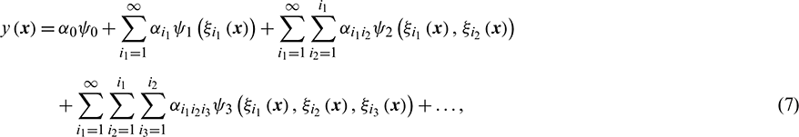
The polynomial chaos expansion is essentially a representation of a function , where is the properly defined probability space. Second-order random processes in [51] are processes with finite variance, and this can be applied to most uncertain event. Thus, a general second-order uncertain process y(x), viewed as a function of x, i.e., the uncertain event, can be represented in the form

where is the polynomial coefficient to be estimated, is the generalized polynomial chaos of order n in terms of the d-dimensional uncertainty variables . For convenience, Eq. (7) is usually expanded and renumbered according to some specific rules, which is simplified in the form of only one index as

where ai and correspond to the polynomial coefficients and basis functions in Eq. (7), respectively.

Note that Eq. (8) is an infinite and convergent summation in the infinite dimensional space of . To reduce computational effort, it is often truncated at the pth-order and rewritten in the following form

where () is the number of retained terms, which is given by

The most important aspect of the above expansions is that an uncertainty process has been decomposed into a set of deterministic functions, and the truncated expansion series, p, mainly depends on the complexity and the nonlinearity of the uncertainty process. A second-order approximation is recommended as a first attempt; this approximation can be refined further using higher order terms, depending on the accuracy needs and available computational resources.

The polynomials satisfy the following orthogonality relation:

where denotes Kronecker delta function, denotes the inner product in the Hilbert space of variables which can be expressed as follows:

Here, is the weight function determined by the distribution of the corresponding uncertainty variables .

3.2 Polynomial Basis Functions for Hybrid Uncertainty Parameters

In Eqs. (8) and (9), the multi-dimensional, hypergeometric polynomials can be expressed as the tensor product of the corresponding one-dimensional polynomials bases:

where denotes the one-dimensional polynomial of the k-dimensional uncertainty variable .

For the stochastic parameters satisfying normal distribution, the one-dimensional polynomial is the Hermite polynomial , which can be expressed as follows:

The ()-th order Hermite polynomial satisfies the following relation:

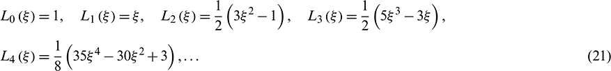
hence the first few Hermite polynomials can be expressed as

The inner product of two Hermite polynomials can be formulated as

where is Kronecker delta function, and

Moreover, the Legendre polynomial is used to describe the interval parameters, which is given by

The ()-th order Legendre polynomial satisfies the following relation:

hence the first few Legendre polynomials can be expressed as

The inner product of two Legendre polynomials can be formulated as

where More polynomial bases, such as Jacobi, Laguerre, and generalized Laguerre polynomials can be found in the relevant literatures [52,53].

3.3 Galerkin Projection Method for the Expansion Coefficients

The Galerkin projection method [13,54] is adopted to identify the coefficient ai in Eq. (8). Applying Galerkin projection, both sides of Eq. (8) are simultaneously projected onto the orthogonal polynomial , such that

Owing to the orthogonality, the expansion coefficient ai in Eq. (8) can be calculated as follows:

It is noted that the denominator term of Eq. (24) is only the inner product of the orthogonal polynomial , which is the tensor product of the corresponding one-dimensional polynomials bases. Hence the denominator term can be regarded as the product of the inner products of the one-dimensional, orthogonal polynomial bases:

where can be easily calculated through Eqs. (17) and (22).

The numerator term of Eq. (24) is determined by calculating the expectation of , which can be expressed as

where is the joint probability density function of . It is noted that this is a numerical integration of multivariate functions, and will be extremely complicated for the complex, nonlinear functions. Here, we use the sparse grid, numerical integration method (SGNIM) [46,55] to compute Eq. (26), while the sparse grid collocation strategy is utilized to generate the integral collocation nodes. For the d-dimensional uncertainty variables , the sparse grid with the k-th collocation level can be expressed as follows:

where is the one-dimensional integral nodes for each uncertain variable; , and id are the multi-indices determining the number of collocation nodes in each dimension (Nj), that is, Nj is a function of ij; k is the collocation level, and larger values of k correspond to higher accuracy. , and the inequality limits to a certain interval, so that all integral collocation nodes satisfying this condition can be found. The detailed formulas are not provided herein; the interested readers are referred to [55].

SGNIM performs the tensor product only on the one-dimensional integration corresponding to the multi-indices that meet , thus avoids the “dimension disaster” caused by the direct tensor product. Such constraint can effectively remove those integral points in the full factor grid [56] that do not contribute significantly to the improvement of accuracy, thereby greatly reducing the computational cost.

Assuming that we obtain a total of N d-dimensional integral collocation nodes through Eq. (27), i.e., , the corresponding integral weight wl of the l-th collocation node can be expressed as follows:

where is the product of the corresponding weights in each dimension of the l-th d-dimensional integral collocation node.

Moreover, the one-dimensional integral node in Eq. (27) and integral weight in Eq. (28) () can be generally calculated through the moment-matching method [57]. For the normal random parameters, and can be easily obtained through Gaussian–Hermite quadrature formula, given by

where and are the integral weights and nodes of Gaussian–Hermite integration, respectively. Similarly, the and of interval parameters can be computed by Gaussian–Legendre quadrature formulas. These weights and nodes of Gaussian quadrature can be easily found in the relevant literature [58], which is not discussed here. Taking the Gaussian–Hermite and Gaussian–Legendre as examples, the sparse grids in 2D space based on Gaussian abscissas are displayed in Fig. 1.

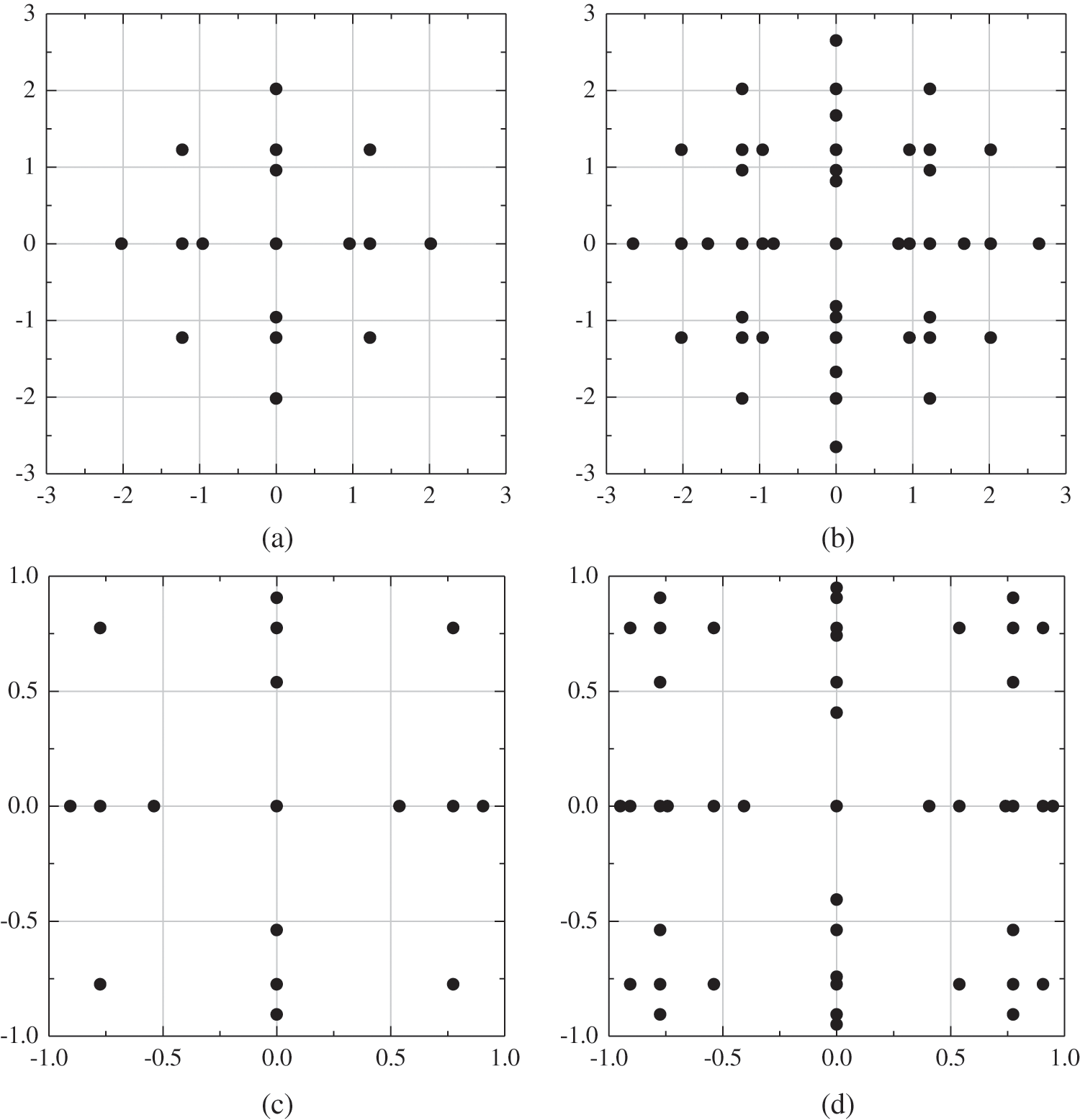
Figure 1: Sparse grids in 2D space based on Gaussian abscissas (a) Gaussian–Hermite, d = 2, k = 2. (b) Gaussian–Hermite, d = 2, k = 3. (c) Gaussian–Legendre, d = 2, k = 2. (d) Gaussian–Legendre, d = 2, k = 3

Using the d-dimensional collocation nodes and the corresponding weights , Eq. (26) can be rewritten as follows:

Then substituting Eqs. (25) and (30) into Eq. (24), we can obtain the expansion coefficient ai.

3.4 Evaluation of the Responses Bounds

After obtaining the PCE model, the statistical moments of the response can be directly derived through the expansion coefficients and the polynomial bases. The mean and standard deviation of can be expressed as follows:

The lower and upper bounds of the response can be determined by the combination of MCS and PCE conveniently. In this process, the first step is to generate the samples of the hybrid uncertainty vector . Then substituting into Eq. (9) to get the responses, we can obtain the probability density function (PDF) of the responses through the samples. In such circumstance, the percentile difference proposed by Du et al. [59] is usually used as an uncertainty measure, defined by

where and are two values of y satisfy the following probability relation:

and are, respectively, the cumulative distribution function (CDF) of y at the left and right tail. For instance, the value of can be taken as 0.05 or 0.01, while the value of can be set as 0.95 or 0.99. is the value of y that corresponds to CDF . Fig. 2 illustrates the concept of the percentile difference. More details can be found in [60].

Figure 2: The concept of the percentile difference

Through the theory of percentile difference, the lower and upper bounds of the response can be regarded as the positions at the left and right tail of its distribution function, satisfying the given CDF (i = 1, 2). Hence the lower and upper bounds of the response can be obtained as follows:

where is the inverse CDF of y.

4  Polynomial Chaos Expansion Approach for Dynamic Response Analysis of Interval ODEs

In this section, the direct MCS for dynamic response analysis will be reviewed briefly, and the polynomial chaos expansion approach for dynamic systems described by ODEs with hybrid uncertainty parameters will be introduced. A numerical example based on the two methods will then be compared to illustrate the advantages of the polynomial chaos expansion approach.

4.1 Direct MCS Method for Dynamic Response Analysis

When using numerical methods to solve the ODEs in Eq. (4), the range of time is discretized into a set of interpolation points (), and the solutions are calculated in turn at each time point. At any time tj, the direct MCS can be used to evaluate the response bounds of the dynamic systems with hybrid stochastic and interval uncertainty. The main solving process is summarized in Fig. 3.

Step 1: Define the numerical solving method for ODEs, the number of samples for MCS, NM, the length of time period, te, the time step, , the CDF of response at the left (right) tail, (), the distribution parameters of stochastic variables, , and the interval bounds of interval variables, .

Step 2: Initialize the cyclic counting indices j = 0 and i = 1, where j and i are introduced to count the iterations of time and the samples, respectively.

Step 3: Generate one group sample of and from their distributions.

Step 4: Take the sample into the original ODEs, and use an appropriate numerical method to calculate the real response at time tj.

Step 5: If i = NM, continue. Else, assume i = i + 1, and go to Step 3.

Step 6: Calculate the statistical moments, and obtain the PDF of the response at time tj through the NM samples.

Step 7: Calculate the response bounds at time tj according to Eqs. (32)–(34).

Step 8: If , output the statistical moments and bounds of dynamic response with time. Else, assume j = j + 1 and i = 1, then go to Step 3.

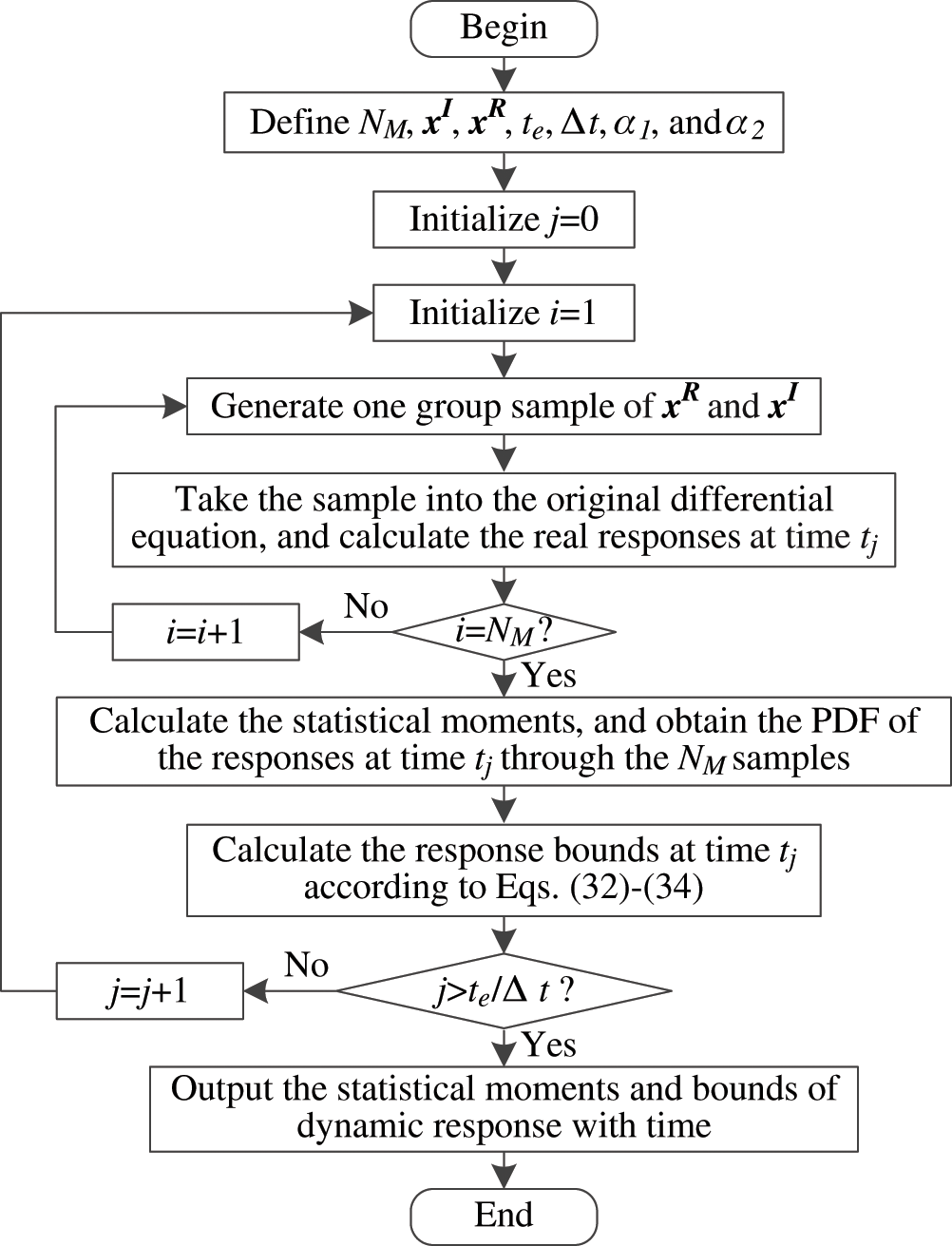
Figure 3: The solving process of the direct MCS method for dynamic response analysis

4.2 The Computational Procedure of the Polynomial Chaos Expansion Approach

At time tj, the dynamic response of the ODEs in Eq. (4) with respect to the hybrid uncertainty vector can be approximated by the truncated polynomial chaos as shown in Eq. (9). The polynomial chaos model is an uncertainty function since the ODEs are with hybrid stochastic and interval parameters. To generate a PCE model at time tj, we must preset the polynomial basis functions according to the distributions of the uncertainty parameters, and specify the expansion series of polynomial chaos as well as the collocation level k in SGNIM. After ai is obtained through the Galerkin projection method, the PCE model is independent of the degree of freedom of the structure and therefore, a computationally efficient surrogate model. In this case, combined with MCS, the response bounds at time tj can be efficiently evaluated with a low computational cost. The flowchart of the solving process is plotted in Fig. 4, which can be described as follows:

Step 1: Define the numerical solving method for ODEs, the expansion series of polynomial chaos, p, the collocation level, k, the number of samples for MCS, NM, the length of time period, te, the time step, , the CDF of response at the left (right) tail, (), the distribution parameters of stochastic variables, , and the interval bounds of interval variables, .

Step 2: Determine the polynomial basis functions according to the distributions of the uncertainty parameters.

Step 3: Utilize the sparse grid collocation strategy to generate the integral collocation nodes and the corresponding integral weights according to Eqs. (27) and (28).

Step 4: Initialize the cyclic counting indices j = 0. j is introduced to count the iterations of time.

Step 5: Take the collocation nodes into the original ODEs, and use an appropriate numerical method to calculate the real responses at time tj.

Step 6: Calculate the expansion coefficient of polynomial chaos through the Galerkin projection method according to Eqs. (23)–(26) and (30) to yield the polynomial chaos at time tj.

Step 7: Calculate the statistical moments of the response at time tj according to Eq. (31).

Step 8: Generate NM group samples of and in the corresponding standard uncertainty spaces.

Step 9: Take the NM group samples into the obtained PCE model, and obtain the approximate responses.

Step 10: Obtain the PDF of the responses at time tj through the NM samples.

Step 11: Calculate the response bounds at time tj according to Eqs. (32)–(34).

Step 12: If , output the statistical moments and bounds of dynamic response with time. Else, assume j = j + 1, and go to Step 5.

Figure 4: The solving process of the polynomial chaos expansion approach for dynamic systems described by ODEs with hybrid uncertainty parameters

In a brief description, the proposed polynomial chaos expansion algorithm for solving the dynamic systems described by ODEs with hybrid stochastic and interval parameters is similar to a type of sampling method. It transforms the original ODEs with uncertainty parameters into ODEs with deterministic parameters through sampling, without changing their expressions. As a non-intrusive method, any numerical methods can be used to solve the differential equations. Thus, the polynomial chaos expansion approach can be regarded as a computationally convenient method.

4.3 A Numerical Example and Discussions

A simple numerical example is used here to demonstrate the validity of the present method. The results obtained by the polynomial chaos method which is abbreviated as PCEM are compared with those of the direct MCS. The schematic of a double pendulum system is analyzed as depicted in Fig. 5. The differential equations of this system can be expressed as follows:

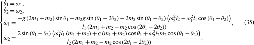
where m1 and m2 are the masses of the two pendulums, respectively; l1 and l2 are the lengths of the pendulum rods, respectively; and (i = 1, 2) are respectively the angles and the angular velocities of the pendulum rods, and g is the gravity acceleration. Here, we assume that m1 and m2 satisfy Gaussian distribution, with the mean and standard deviation of 1.0 and 0.1 kg, respectively. Note that Gaussian distribution is unbounded distribution with infinite interval, it means that the parameter values will be negative to some extent. Therefore, the modeling of stochastic variables is an approximate situation. l1 and l2 are considered as interval parameters, and their interval ranges are [0.45, 0.55] m, and [0.9, 1, 1] m, respectively. The initial conditions are [, , 0, 0].

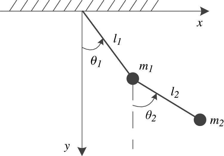
Figure 5: The schematic of a double pendulum system

For this problem, the fifth-order polynomial chaos approach is used to solve the differential equations in the time period of 0–10 s. The collocation level k in SGNIM is set as 4, thus the total number of samples in PCEM are 999, and the number of samples for MCS is 10000. The direct MCS is used to generate the reference solutions for comparison, in which the sample size is 10000. Moreover, and in the two algorithms are set as 0.001 and 0.999, respectively. The results of the angles and the angular velocities of the two pendulum rods are plotted in Figs. 6 and 7, respectively. To show it in a more intuitive way, detailed information of the angular velocities of the first and second pendulum rods are listed in Tabs. 1 and 2 at 10 time instants from 1 to 10 s. All calculations are completed on a desktop personal computer with 16 GB RAM and a CPU core of Intel(R) Core(TM) i5-4590 CPU clocked at 3.30 GHz.

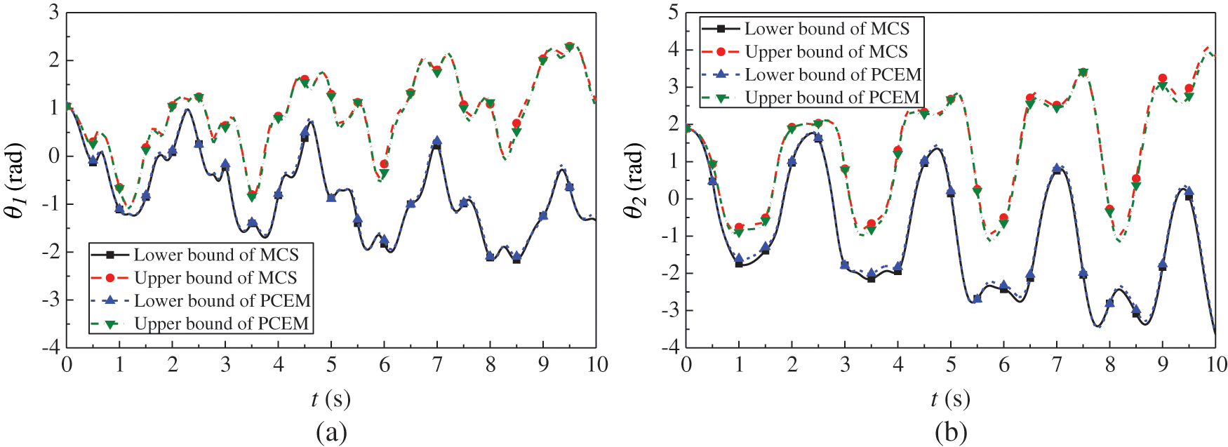
Figure 6: The response bounds of the angles in a time period 10 s (a) the angle of the first pendulum rod (b) the angle of the second pendulum rod

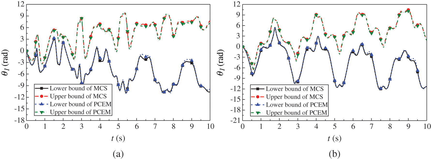
Figure 7: The bounds of the angular velocities in a time period 10 s (a) the angular velocity of the first pendulum rod (b) the angular velocity of the second pendulum rod

Table 1: The detailed information of (rad/s) in a time period 10 s

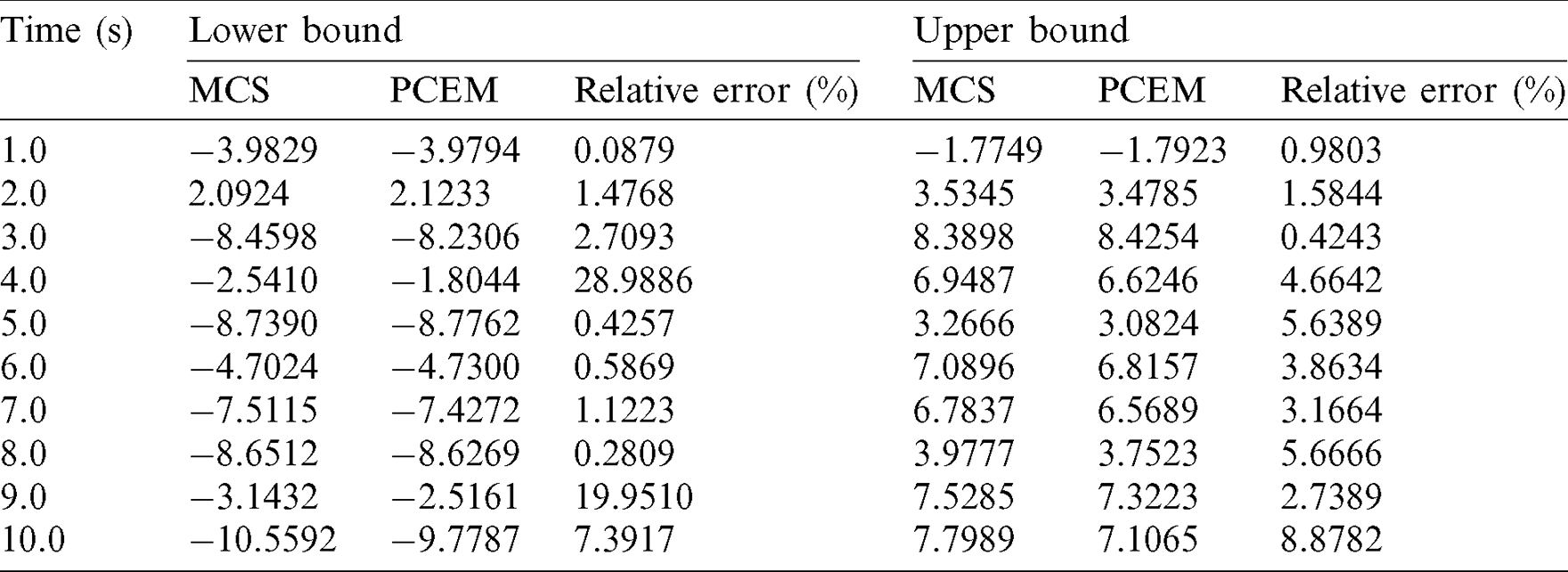
Table 2: The detailed information of (rad/s) in a time period 10 s

As shown in Figs. 6 and 7 and Tabs. 1 and 2, the response bounds of the double pendulum system yielded by PCEM almost match the results of the direct MCS in most time period. Therefore, we can summarize that the PCEM can be considered as an alternative algorithm with fine precision when calculating the response bounds of dynamic systems with hybrid stochastic and interval uncertainty. Furthermore, Figs. 6 and 7 show that the ranges of the upper and lower bounds of , , , and gradually expand with time. The dynamic responses of the double pendulum system are very sensitive to the uncertainty parameters. Therefore, the uncertainty of the dynamic response deserves more attention in structure design and analysis.

Moreover, the computations of PCEM and direct MCS take 128.67 s and 1347.42 s, respectively. Clearly, the computational efficiency of PCEM is much higher than that of the direct MCS. Therefore, the proposed method can be considered as an effective and efficient uncertainty analysis method for the dynamic systems with hybrid stochastic and interval uncertainty parameters.

5  The Uncertainty Analysis of Artillery Exterior Ballistic Dynamics

The schematic of the artillery exterior ballistic dynamics model is analyzed as depicted in Fig. 8. The artillery exterior ballistic is the most typical uncertainty process in the artillery launching process, which is affected by various uncertainties such as propellant parameters, projectile characteristic parameters, artillery muzzle vibration, meteorological environment, operation error, and so on. These uncertainties will inevitably affect the final dynamics performance, thus the flight trajectory and motion attitude of each projectile is different. These differences eventually converge to the projectile impact point, and affect a very important tactical indicator of artillery system, namely artillery firing dispersion. The existence of uncertainties is the primary cause projectile dispersion. The uncertainty analysis of artillery exterior ballistic dynamics model can explore the impact of the uncertainty parameters on the projectile flight, which is of great significance for achieving effective control of the artillery firing dispersion.

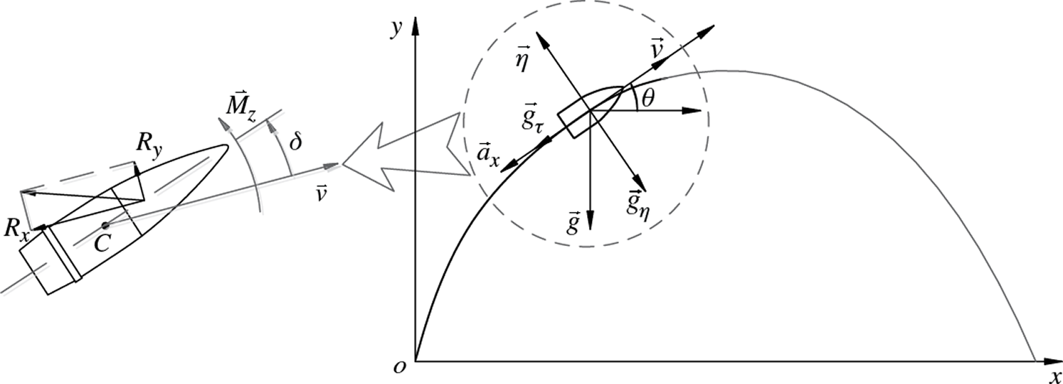
Figure 8: The schematic of the artillery exterior ballistic dynamics model

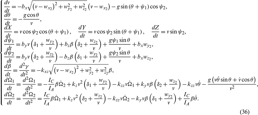
A general six-degree of freedom exterior ballistic model can be formulated as follows:

where v is the projectile velocity, is the path angle, and are, respectively, the vertical and the horizontal deflection angle; (X, Y, Z) indicate the position of centroid of the projectile in the ground coordinate corresponding to the firing distance, height, and offset, respectively; and are, respectively, the vertical and horizontal attack angle; is the rotation angle, and is the rotation angular velocity; and are the vertical and the horizontal angle of oscillation, respectively, while and are the corresponding angular velocities; IC is the polar moment of inertia; IA is the equatorial moment of inertia; bx, by, bz, kxz, kzz, ky, and kz are the aerodynamic parameters of the projectile, which are related to the shape and size of the projectile, such as the projectile mass mp, the maximum diameter of projectile dmax, and the distance from the projectile centroid to its top lcg. Detailed auxiliary equations of the aerodynamic parameters can be found in [61]. wx2, wy2, and wz2 are the projections of wind speed on the velocity coordinate, which are given by

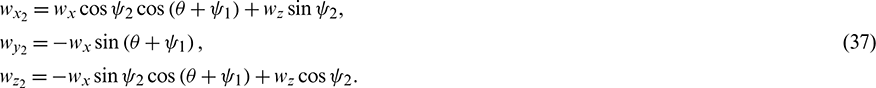
where wx and wz are the longitudinal wind and the horizontal wind, respectively.

Through the above equations, we can obtain the flight trajectory and motion attitude of the projectile. Assuming that there are uncertain parameters in this dynamics model, the detailed uncertainty types and values are shown in Tab. 3. This process has a total of 14 uncertainty parameters, which is a typical, high-dimensional, uncertainty analysis problem.

Table 3: Uncertainty parameters for an exterior ballistic model

The second-order polynomial chaos approach is used to solve the differential equations in the time period of 0–107 s. The collocation level k in SGNIM is set as 2, thus the sample size for PCEM is 632, and the number of samples for MCS is 10000. The direct MCS is used to generate the reference solutions for comparison, in which the sample size is 10000. and in the two algorithms are set as 0.001 and 0.999, respectively. Partial results including the velocity v, the rotation angular velocity , and the horizontal deflection angle of the projectile are shown in Fig. 9. Detailed information of v and is listed in Tabs. 4 and 5, respectively. Moreover, Fig. 10 gives the spatial ranges of the projectile flight trajectory.

Figure 9: The response bounds of an artillery exterior ballistic dynamics model in a time period 107 s (a) the velocity of the projectile (b) the rotation angular velocity of the projectile (c) the horizontal deflection angle of the projectile

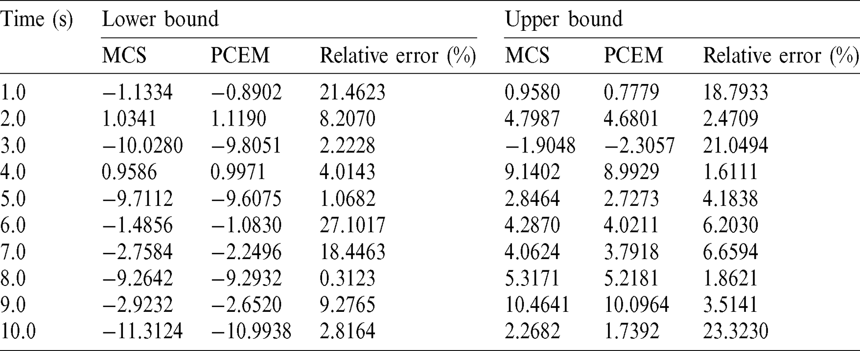
Table 4: The detailed information of v (m/s) in a time period 107 s

Table 5: The detailed information of (rad) in a time period 107 s

Figure 10: The spatial ranges of the projectile flight trajectory (a) flight trajectory bounds in ground coordinate (b) projection of projectile flight in XZ plane

Figs. 9 and 10 show that the response bounds of the artillery exterior ballistic dynamics model yielded by PCEM perfectly match the results of the direct MCS perfectly, which is further indicated intuitively by Tabs. 4 and 5. Moreover, it is noted that the number of hybrid uncertainty parameters is up to 14. The results show that the proposed method has fine precision even in the high-dimensional, uncertainty problem. Furthermore, the computational time of direct MCS is 124879.612 s, while the computing time of PCEM is only 4521.29 s. This example demonstrates that high precision and low computational cost can be achieved by the proposed method when calculating the response bounds of artillery dynamics with hybrid stochastic and interval uncertainty.

Furthermore, Fig. 9 shows that the dynamic behaviors obtained by the proposed method are ranges rather than deterministic ones. It fully reflects the fluctuation of these dynamic behaviors caused by uncertainty. Hence the upper and lower bounds of these dynamic behaviors can provide a good reference for the artillery exterior ballistic design. More importantly, the uncertainty analysis of artillery external ballistic dynamics can predict the projectile flight trajectory under uncertain parameters. Fig. 10a gives the spatial ranges of the projectile flight trajectory derived by the two methods, and the shadow area in Fig. 10b is the possible range of the projectile impact point, so that the projectile dispersion caused by uncertainty parameters can be predicted.

6  Conclusions

In this paper, a hybrid stochastic and interval uncertainty analysis method with polynomial chaos expansion is proposed to evaluate the response bounds of artillery dynamics. In this method, the Hermite polynomial in stochastic space and the Legendre polynomial in interval space are employed, respectively, as the trial basis to expand the Gaussian and interval processes. The polynomial coefficients are calculated through the Galerkin projection method, in which the sparse grid, numerical integration method is used to generate the integral points and the corresponding integral weights. Through the sampling in polynomial chaos expansion, the original artillery dynamics systems with hybrid stochastic and interval parameters can be transformed into ones with deterministic parameters, without changing their expressions. The yielded polynomial chaos expansion model is utilized as a computationally efficient surrogate model, and the supremum and infimum of the dynamic responses at each iteration time step can be easily approximated through Monte Carlo simulation and percentile difference. A numerical example and an artillery exterior ballistic dynamics model were used to illustrate the feasibility and efficiency of this approach. The numerical results indicate that the dynamic response bounds obtained by the polynomial chaos expansion approach almost match the results of the direct Monte Carlo simulation, but the computational efficiency of the polynomial chaos expansion approach is much higher than direct Monte Carlo simulation. Moreover, the proposed method also exhibits fine precision even in high-dimensional uncertainty analysis problems. Another advantage of the polynomial chaos expansion approach is that it is non-intrusive. In a brief description, the proposed algorithm is similar to a type of sampling method. It has no special restrictions on numerical methods for solving the differential equations. Therefore, this method can be potentially applied to other artillery dynamics systems with hybrid uncertainty parameters, such as the artillery multi-body dynamics system described by the differential-algebraic equations (DAEs). However, further research is required to explore the potential of the proposed method in dealing with other artillery dynamics system.

Funding Statement: This research was financially supported by the National Natural Science Foundation of China [Grant Nos. 301070603 and 11572158]. Besides, the authors wish to express their many thanks to the reviewers for their useful and constructive comments.

Conflicts of Interest: The authors declare that they have no conflict of intrest to report regarding the present study.

References

 1.  Astill, C. J., Imosseir, S. B., Shinozuka, M. (2007). Impact loading on structures with random properties. Journal of Structural Mechanics, 1(1), 63–77. DOI 10.1080/03601217208905333. [Google Scholar] [CrossRef]

 2.  Segin, A., Dunne, J. F., Zoghaib, L. (2012). Extreme-value-based statistical bounding of low, mid, and high frequency responses of a forced plate with random boundary conditions. Journal of Vibration and Acoustics, 134(2), 021003. DOI 10.1115/1.4005019. [Google Scholar] [CrossRef]

 3.  Rajabalinejad, M., Meester, L. E., Van Gelder, P. H. A. J. M., Vrijling, J. K. (2011). Dynamic bounds coupled with Monte Carlo simulations. Reliability Engineering & System Safety, 96(2), 278–285. DOI 10.1016/j.ress.2010.07.006. [Google Scholar] [CrossRef]

 4.  Chang, T. P., Chang, H. C. (1994). Stochastic dynamic finite element analysis of a nonuniform beam. International Journal of Solids and Structures, 31(5), 587–597. DOI 10.1016/0020-7683(94)90139-2. [Google Scholar] [CrossRef]

 5.  Lei, Z., Qiu, C. (2000). Neumann dynamic stochastic finite element method of vibration for structures with stochastic parameters to random excitation. Computers & Structures, 77(6), 651–657. DOI 10.1016/S0045-7949(00)00019-5. [Google Scholar] [CrossRef]

 6.  Guerine, A., El Hami, A., Walha, L., Fakhfakh, T., Haddar, M. (2015). A perturbation approach for the dynamic analysis of one stage gear system with uncertain nnparameters. Mechanism and Machine Theory, 92, 113–126. DOI 10.1016/j.mechmachtheory.2015.05.005. [Google Scholar] [CrossRef]

 7.  Wan, H. P., Mao, Z., Todd, M. D., Ren, W. X. (2014). Analytical uncertainty quantification for modal frequencies with structural parameter uncertainty using a Gaussian process metamodel. Engineering Structures, 75, 577–589. DOI 10.1016/j.engstruct.2014.06.028. [Google Scholar] [CrossRef]

 8.  Wan, H. P., Ren, W. X., Todd, M. D. (2017). An efficient metamodeling approach for uncertainty quantification of complex systems with arbitrary parameter probability distributions. International Journal for Numerical Methods in Engineering, 109(5), 739–760. DOI 10.1002/nme.5305. [Google Scholar] [CrossRef]

 9.  Lu, J., Zhan, Z., Apley, D. W., Chen, W. (2019). Uncertainty propagation of frequency response functions using a multi-output Gaussian process model. Computers & Structures, 217, 1–17. DOI 10.1016/j.compstruc.2019.03.009. [Google Scholar] [CrossRef]

10. Ngah, M. F., Young, A. (2007). Application of the spectral stochastic finite element method for performance prediction of composite structures. Composite Structures, 78(3), 447–456. DOI 10.1016/j.compstruct.2005.11.009. [Google Scholar] [CrossRef]

11. Nouy, A. (2009). Recent developments in spectral stochastic methods for the numerical solution of stochastic partial differential equations. Archives of Computational Methods in Engineering, 16(3), 251–285. DOI 10.1007/s11831-009-9034-5. [Google Scholar] [CrossRef]

12. Tootkaboni, M., Graham–Brady, L. (2010). A multi-scale spectral stochastic method for homogenization of multi-phase periodic composites with random material properties. International Journal for Numerical Methods in Engineering, 83(1), 59–90. DOI 10.1002/nme.2829. [Google Scholar] [CrossRef]

13. Xiu, D., Karniadakis, G. E. (2002). The Wiener-Askey polynomial chaos for stochastic differential equations. SIAM Journal on Scientific Computing, 24(2), 619–644. DOI 10.1137/S1064827501387826. [Google Scholar] [CrossRef]

14. Creamer, D. B. (2006). On using polynomial chaos for modeling uncertainty in acoustic propagation. Journal of the Acoustical Society of America, 119(4), 1979–1994. DOI 10.1121/1.2173523. [Google Scholar] [CrossRef]

15. Ghanem, R., Masri, S., Pellissetti, M., Wolfe, R. (2005). Identification and prediction of stochastic dynamical systems in a polynomial chaos basis. Computer Methods in Applied Mechanics and Engineering, 194(12–16), 1641–1654. DOI 10.1016/j.cma.2004.05.031. [Google Scholar] [CrossRef]

16. Sandu, A., Sandu, C., Ahmadian, M. (2006). Modeling multibody systems with uncertainties. Part I: Theoretical and computational aspects. Multibody System Dynamics, 15(4), 369–391. DOI 10.1007/s11044-006-9007-5. [Google Scholar] [CrossRef]

17. Sandu, C., Sandu, A., Ahmadian, M. (2006). Modeling multibody systems with uncertainties. Part II: Numerical applications. Multibody System Dynamics, 15(3), 241–262. DOI 10.1007/s11044-006-9008-4. [Google Scholar] [CrossRef]

18. Saha, S. K., Sepahvand, K., Matsagar, V. A., Jain, A. K., Marburg, S. (2013). Stochastic analysis of base-isolated liquid storage tanks with uncertain isolator parameters under random excitation. Engineering Structures, 57, 465–474. DOI 10.1016/j.engstruct.2013.09.037. [Google Scholar] [CrossRef]

19. Wan, H. P., Ren, W. X., Todd, M. D. (2020). Arbitrary polynomial chaos expansion method for uncertainty quantification and global sensitivity analysis in structural dynamics. Mechanical Systems and Signal Processing, 142, 106732. DOI 10.1016/j.ymssp.2020.106732. [Google Scholar] [CrossRef]

20. Alefeld, G., Mayer, G. (2000). Interval analysis: Theory and applications. Journal of Computational and Applied Mathematics, 121(1–2), 421–464. DOI 10.1016/S0377-0427(00)00342-3. [Google Scholar] [CrossRef]

21. Gao, W. (2007). Natural frequency and mode shape analysis of structures with uncertainty. Mechanical Systems and Signal Processing, 21(1), 24–39. DOI 10.1016/j.ymssp.2006.05.007. [Google Scholar] [CrossRef]

22. Moens, D., Vandepitte, D. (2005). A survey of non-probabilistic uncertainty treatment in finite element analysis. Computer Methods in Applied Mechanics and Engineering, 194(12–16), 1527–1555. DOI 10.1016/j.cma.2004.03.019. [Google Scholar] [CrossRef]

23. Makino, K., Berz, M. (2006). Suppresion of the wrapping effect by Taylor model-based verified integrators: Long-term stabilization by shrink wrapping. International Journal of Differential Equations and Applications, 10(4), 385–403. [Google Scholar]

24. Makino, K., Berz, M. (1999). Efficient control of the dependency problem based on Taylor model methods. Reliable Computing, 5(1), 3–12. DOI 10.1023/A:1026485406803. [Google Scholar] [CrossRef]

25. Lin, Y., Stadtherr, M. A. (2007). Validated solutions of initial value problems for parametric ODEs. Applied Numerical Mathematics, 57(10), 1145–1162. DOI 10.1016/j.apnum.2006.10.006. [Google Scholar] [CrossRef]

26. Xia, Y., Qiu, Z., Friswell, M. I. (2010). The time response of structures with bounded parameters and interval initial conditions. Journal of Sound and Vibration, 329(3), 353–365. DOI 10.1016/j.jsv.2009.09.019. [Google Scholar] [CrossRef]

27. Liu, N., Gao, W., Song, C., Zhang, N., Pi, Y. L. (2013). Interval dynamic response analysis of vehicle-bridge interaction system with uncertainty. Journal of Sound and Vibration, 332(13), 3218–3231. DOI 10.1016/j.jsv.2013.01.025. [Google Scholar] [CrossRef]

28. Qiu, Z., Wang, X. (2003). Comparison of dynamic response of structures with uncertain-but-bounded parameters using non-probabilistic interval analysis method and probabilistic approach. International Journal of Solids and Structures, 40(20), 5423–5439. DOI 10.1016/S0020-7683(03)00282-8. [Google Scholar] [CrossRef]

29. Qiu, Z., Wang, X. (2005). Parameter perturbation method for dynamic responses of structures with uncertain-but-bounded parameters based on interval analysis. International Journal of Solids and Structures, 42(18–19), 4958–4970. DOI 10.1016/j.ijsolstr.2005.02.023. [Google Scholar] [CrossRef]

30. Zhang, X. M., Ding, H., Chen, S. H. (2007). Interval finite element method for dynamic response of closed-loop system with uncertain parameters. International Journal for Numerical Methods in Engineering, 70(5), 543–562. DOI 10.1002/nme.1891. [Google Scholar] [CrossRef]

31. Han, X., Jiang, C., Gong, S., Huang, Y. H. (2008). Transient waves in composite-laminated plates with uncertain load and material property. International Journal for Numerical Methods in Engineering, 75(3), 253–274. DOI 10.1002/nme.2248. [Google Scholar] [CrossRef]

32. Qiu, Z., Elishakoff, I. (1998). Antioptimization of structures with large uncertain-but-non-random parameters via interval analysis. Computer Methods in Applied Mechanics and Engineering, 152(3–4), 361–372. DOI 10.1016/S0045-7825(96)01211-X. [Google Scholar] [CrossRef]

33. Wu, J., Zhang, Y., Chen, L., Luo, Z. (2013). A Chebyshev interval method for nonlinear dynamic systems under uncertainty. Applied Mathematical Modelling, 37(6), 4578–4591. DOI 10.1016/j.apm.2012.09.073. [Google Scholar] [CrossRef]

34. Wan, H. P., Ni, Y. Q. (2020). A new approach for interval dynamic analysis of train-bridge system based on Bayesian optimization. Journal of Engineering Mechanics, 146(5), 4020029. DOI 10.1061/(ASCE)EM.1943-7889.0001735. [Google Scholar] [CrossRef]

35. Moens, D., Vandepitte, D. (2006). Recent advances in non-probabilistic approaches for non-deterministic dynamic finite element analysis. Archives of Computational Methods in Engineering, 13(3), 389–464. DOI 10.1007/BF02736398. [Google Scholar] [CrossRef]

36. Cacciola, P., Muscolino, G., Versaci, C. (2011). Deterministic and stochastic seismic analysis of buildings with uncertain-but-bounded mass distribution. Computers & Structures, 89(21–22), 2028–2036. DOI 10.1016/j.compstruc.2011.05.017. [Google Scholar] [CrossRef]

37. Muscolino, G., Sofi, A. (2011). Response statistics of linear structures with uncertain-but-bounded parameters under Gaussian stochastic input. International Journal of Structural Stability and Dynamics, 11(4), 775–804. DOI 10.1142/S0219455411004348. [Google Scholar] [CrossRef]

38. Muscolino, G., Sofi, A. (2012). Stochastic analysis of structures with uncertain-but-bounded parameters via improved interval analysis. Probabilistic Engineering Mechanics, 28, 152–163. DOI 10.1016/j.probengmech.2011.08.011. [Google Scholar] [CrossRef]

39. Xia, B., Yu, D., Liu, J. (2013). Hybrid uncertain analysis of acoustic field with interval random parameters. Computer Methods in Applied Mechanics and Engineering, 256, 56–69. DOI 10.1016/j.cma.2012.12.016. [Google Scholar] [CrossRef]

40. Xia, B., Yu, D., Liu, J. (2013). Hybrid uncertain analysis for structural-acoustic problem with random and interval parameters. Journal of Sound and Vibration, 332(11), 2701–2720. DOI 10.1016/j.jsv.2012.12.028. [Google Scholar] [CrossRef]

41. Chen, N., Yu, D., Xia, B. (2014). Hybrid uncertain analysis for the prediction of exterior acoustic field with interval and random parameters. Computers & Structures, 141, 9–18. DOI 10.1016/j.compstruc.2014.05.004. [Google Scholar] [CrossRef]

42. Xia, B., Yin, S., Yu, D. (2015). A new random interval method for response analysis of structural-acoustic system with interval random variables. Applied Acoustics, 99, 31–42. DOI 10.1016/j.apacoust.2015.05.002. [Google Scholar] [CrossRef]

43. Xia, B., Yu, D. (2014). Change-of-variable interval stochastic perturbation method for hybrid uncertain structural-acoustic systems with random and interval variables. Journal of Fluids and Structures, 50, 461–478. DOI 10.1016/j.jfluidstructs.2014.07.005. [Google Scholar] [CrossRef]

44. Xia, B., Yu, D., Han, X., Jiang, C. (2014). Unified response probability distribution analysis of two hybrid uncertain acoustic fields. Computer Methods in Applied Mechanics and Engineering, 276, 20–34. DOI 10.1016/j.cma.2014.03.014. [Google Scholar] [CrossRef]

45. Wang, M., Huang, Q. (2016). A new hybrid uncertain analysis method for structural-acoustic systems with random and interval parameters. Computers & Structures, 175, 15–28. DOI 10.1016/j.compstruc.2016.07.001. [Google Scholar] [CrossRef]

46. Xu, M., Du, J., Wang, C., Li, Y. (2017). Hybrid uncertainty propagation in structural-acoustic systems based on the polynomial chaos expansion and dimension-wise analysis. Computer Methods in Applied Mechanics and Engineering, 320, 198–217. DOI 10.1016/j.cma.2017.03.026. [Google Scholar] [CrossRef]

47. Wu, J., Luo, Z., Zhang, N., Zhang, Y. (2015). A new uncertain analysis method and its application in vehicle dynamics. Mechanical Systems and Signal Processing, 50–51, 659–675. DOI 10.1016/j.ymssp.2014.05.036. [Google Scholar] [CrossRef]

48. Wang, M., Wan, Z., Huang, Q. (2016). A new uncertain analysis method for the prediction of acoustic field with random and interval parameters. Shock and Vibration, 2016, 3693262. DOI 10.1155/2016/3693262. [Google Scholar] [CrossRef]

49. Wang, L., Yang, G., Xiao, H., Sun, Q., Ge, J. (2020). Interval optimization for structural dynamic responses of an artillery system under uncertainty. Engineering Optimization, 52(2), 343–366. DOI 10.1080/0305215X.2019.1590563. [Google Scholar] [CrossRef]

50. Wiener, N. (1938). The Homogeneous chaos. American Journal of Mathematics, 60(4), 897. DOI 10.2307/2371268. [Google Scholar] [CrossRef]

51. Cameron, R. H., Martin, W. T. (1947). The orthogonal development of non-linear functionals in series of Fourier-Hermite functionals. Annals of Mathematics, 48(2), 385. DOI 10.2307/1969178. [Google Scholar] [CrossRef]

52. Xiu, D., Hesthaven, J. S. (2005). High-order collocation methods for differential equations with random inputs. SIAM Journal on Scientific Computing, 27(3), 1118–1139. DOI 10.1137/040615201. [Google Scholar] [CrossRef]

53. Xiu, D. (2010). Numerical methods for stochastic computations: A spectral method approach. New Jersey, USA: Princeton University Press. [Google Scholar]

54. Xiu, D., Karniadakis, G. E. (2003). Modeling uncertainty in flow simulations via generalized polynomial chaos. Journal of Computational Physics, 187(1), 137–167. DOI 10.1016/S0021-9991(03)00092-5. [Google Scholar] [CrossRef]

55. Gerstner, T., Griebel, M. (1998). Numerical integration using sparse grids. Numerical Algorithms, 18(3/4), 209–232. DOI 10.1023/A:1019129717644. [Google Scholar] [CrossRef]

56. Seo, H. S., Kwak, B. M. (2010). Efficient statistical tolerance analysis for general distributions using three-point information. International Journal of Production Research, 40(4), 931–944. DOI 10.1080/00207540110095709. [Google Scholar] [CrossRef]

57. Lee, S. H., Choi, H. S., Kwak, B. M. (2008). Multilevel design of experiments for statistical moment and probability calculation. Structural and Multidisciplinary Optimization, 37(1), 57–70. DOI 10.1007/s00158-007-0215-2. [Google Scholar] [CrossRef]

58. Abramowitz, M., Stegun, I. A. (1965). Handbook of mathematical functions: With formulas, graphs, and mathematical tables. USA: Dover Publications. [Google Scholar]

59. Du, X., Sudjianto, A., Chen, W. (2004). An integrated framework for optimization under uncertainty using inverse reliability strategy. Journal of Mechanical Design, 126(4), 562–570. DOI 10.1115/1.1759358. [Google Scholar] [CrossRef]

60. Huang, B., Du, X. (2007). Analytical robustness assessment for robust design. Structural and Multidisciplinary Optimization, 34(2), 123–137. DOI 10.1007/s00158-006-0068-0. [Google Scholar] [CrossRef]

61. Han, Z. (2014). Exterior ballistics of projectiles and rockets. Beijing, China: Beijing Institute of Technology Press. [Google Scholar]

This work is licensed under a Creative Commons Attribution 4.0 International License, which permits unrestricted use, distribution, and reproduction in any medium, provided the original work is properly cited.