Computer Modeling in Engineering & Sciences

DOI: 10.32604/cmes.2021.012575

ARTICLE

A Meshless Collocation Method with Barycentric Lagrange Interpolation for Solving the Helmholtz Equation

Miaomiao Yang, Wentao Ma and Yongbin Ge*

Institute of Applied Mathematics and Mechanics, Ningxia University, Yinchuan, 750021, China
*Corresponding Author: Yongbin Ge. Email: gyb@nxu.edu.cn
Received: 05 July 2020; Accepted: 21 September 2020

1  Introduction

In the present work, we consider the following two-dimensional Helmholtz equation:

where is the problem region, is an unknown function of x and y. is the wave number, which could be either a constant or a function of x and y. is a source term. The Dirichlet boundary conditions are given as:

Helmholtz equation is an elliptical partial differential equation, which represents the solution of the wave equation independent of time and it arises from time-harmonic wave propagation [1]. This equation can simulate a variety of physical phenomena, including vibration analysis, water wave propagation, electromagnetic scattering, acoustic scattering, and radar scattering, etc. [2–6]. There is a long history about the development of wave propagation [7]. When the wavenumber is large, the solution of Helmholtz equation is highly oscillatory, so there are some difficulties in obtaining the numerical solution. Meanwhile, because of the complexity of variable wave number Helmholtz equation, it also brings great difficulties to numerical calculation, which still need to be further studied. Therefore, the research on numerical solution method of Helmholtz equation has important theoretical value and practical significance. A variety of numerical methods have been developed to solve the Helmholtz equation, such as the finite element method, boundary element method, finite difference method, meshless method and so on [8–11]. Among them, the finite element method is the most widely used method, but the calculation accuracy of the finite element method will sharply reduce with the increase of the wave number of the equation. At the same time, the meshless method is favored by many researchers because of its many advantages, such as simple discretization, easy derivation of format, easy realization of calculation program, high calculation accuracy and good numerical stability.

A new boundary method with method of external sources for eigenproblems was presented by Reutskiy [12] to solve Helmholtz equation in simply and multiply connected domains. However, this method depends on the grid, so when it applied to eigenproblem in irregular region, meshless technique is needed. Chen et al. [13] put forward a first-order system least square method for solving high wave number problems, and then a nontrivial decomposition is used to solve the first-order system least square problem, which was a new method different from the standard finite element method. Dogan et al. [14] studied the dispersion error of the Helmholtz equation by using the local meshless boundary integral equation method and the radial basis integral equation method. Both methods used the second-order polynomial and the frequency dependent radial basis function to interpolate the potential field, which can solve the high wave number problems. But the cost is to solve a larger linear system, which is computationally intensive. Based on the meshless and boundless analysis of Helmholtz equation, Chen et al. [15] proposed a boundless Burton Miller method by using Burton Miller formula. This method can find the unique solution for all wave numbers, and can also deal with Helmholtz equation under the high wave numbers. However, the cost of calculation is expensive and the derivation process is complicated. Qu et al. [16] developed a local basic solution method which was different from the traditional basic solution method. According to the nodes, the calculation domain was divided into several overlapping subdomains. Finally, the sparse strip matrix was used to solve large-scale problems. Whereas, the numerical implementation is complicated. By using an asymptotic expansion that removes the singularities up to several leading orders, Britt et al. [17] put forward a method that can keep high order convergence even if there is singular solution for Helmholtz equation. Whereas, it did not give out the results in the case of large wave number. A circular boundary knot method was studied by Lin et al. [18] by placing the collocation nodes on the boundary surface in a circular form to solve the high wave number Helmholtz equation, the BKM matrix obtained has the block structure of cyclic matrix and can be solved effectively. Which needs to solve a lot of small matrices, the calculation storage capacity is large. Wang et al. [19] considered the Helmholtz equation in the outer domain, and proposed a finite difference scheme in polar or spherical coordinates, which can solve high wave number problems. Whereas, the “pollution effect” in the domain of the origin of coordinates is inevitable. In addition, the common disadvantage of the above literature is that there is few mention of the case of variable wave number problem.

In this paper, based on the Chebyshev nodes, the scheme for solving the Helmholtz equation is derived by using barycentric Lagrange interpolation basis function. This method is simple in theory, needs few interpolation nodes, and the final discrete matrix is easy to be dealt with. It can not only calculate the high wave number problems, but also calculate the variable wave number problems. It has the advantages including short calculation time, high accuracy and good stability. In this meshless method, the point collocation technique is used for forming the final system of linear algebraic equations. Thus, the present method is a variant of the well-known finite point method [20]. And another analogous method is the localized method of fundamental solutions [21]. The remainder of this paper is arranged as follows: in Section 2, the calculation formula of the two-dimensional barycentric Lagrange interpolation and some theoretical knowledge of the simplified matrix are introduced. In Section 3, the interpolation collocation method and its discrete matrix for calculating the two-dimensional Helmholtz Eq. (1.1) are derived. In Section 4, the numerical results for some test problems are given and compared with the results in the literature. Finally, conclusions are included in Section 5.

2  Barycentric Lagrange Interpolation

2.1 Barycentric Lagrange Interpolation Formula

Let be a given interpolation node, and the corresponding function value is fi, then Lagrange polynomial interpolation formula can be expressed as

where is Lagrange interpolation basis function in the form of

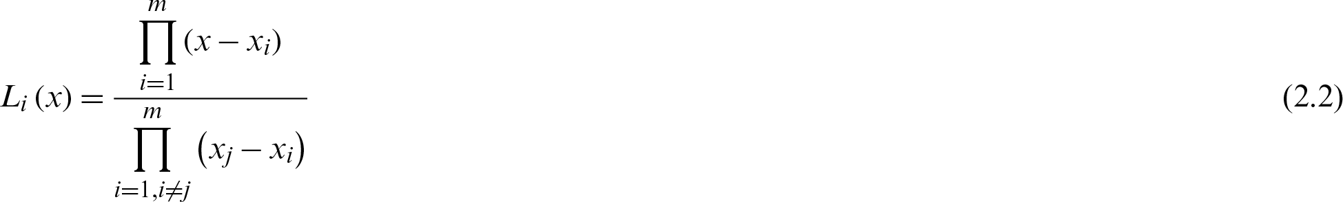
According to Eq. (2.1), it can be concluded that when new interpolation nodes are added, the interpolation basis function needs to be recalculated, which increases the calculation amount. However, if we start from the basis function and extract the common part, its expression will be changed and the calculation amount will be reduced consequently.

Set

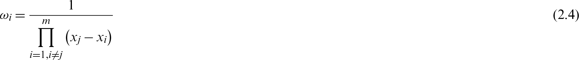
Defines weight of the barycentric Lagrange interpolation function as

As usual, we can get the following algorithm flow diagram (see Fig. 1) for computing

Figure 1: The algorithm flow diagram of

Then, the interpolation basis function (2.2) can be changed to

Substitute Eq. (2.5) into Eq. (2.1) to get

The Eq. (2.6) is called the improved Lagrange interpolation formula [22]. The part of main improvement is to construct Eq. (2.3), thus rewriting the interpolation basis function Eq. (2.2) into the form of Eq. (2.5). The purpose is with number of Lagrange interpolation nodes increases, the computation amount decreases a lot, from to .

By using Eq. (2.6) to interpolate the constant 1 with then we have

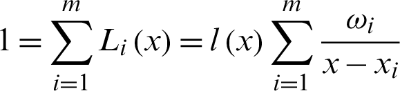
After simplification, it can be obtained

Substituting Eq. (2.7) into Eq. (2.6), we have

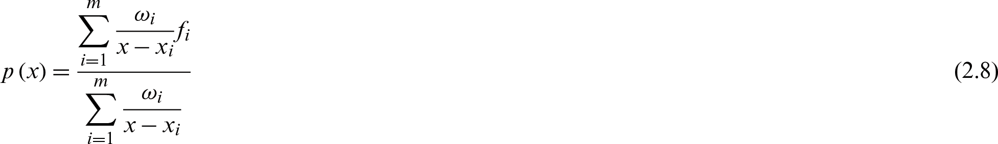
The Eq. (2.8) is called the barycentric Lagrange interpolation formula [22]. Compared with Eq. (2.6), Eq. (2.8) overcomes the Runge phenomenon effectively while maintaining the same computational cost .

2.2 Bivariate Barycenter Lagrange Interpolation Formula

Let the be a function about the variable x and y, and define the interval as . When the interval and is discretized into m and n nodes, respectively, then there are tensor product interpolation nodes in the whole domain . Then the barycentric Lagrange interpolation formula [23] of the is

where 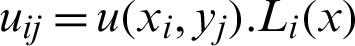and Mj(y) are the interpolation basis functions in the x and y direction, respectively.

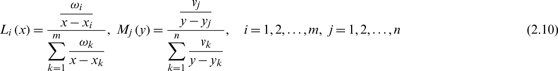
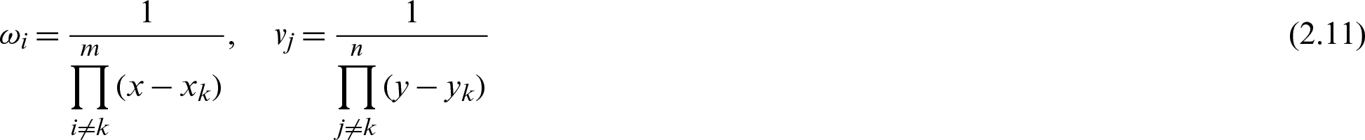
where the weight is

2.3 Interpolation Knot

We can see from the expression of the barycentric Lagrange interpolation weight function Eqs. (2.4) or (2.11) that the selection of the interpolation weight is only related to the distribution of the nodes. Therefore we consider the three kinds of nodes as interpolation nodes and test nodes. They are random nodes, uniform nodes and Chebyshev nodes. Because random nodes and uniforms nodes can be directly implemented in programming language, this part only gives the Chebyshev nodes formula:

Chebyshev nodes of the first kind:

Chebyshev nodes of the second kind:

What needs to be explained is that for two types of Chebyshev node formulas, the defined interval is As for the general interval the coordinate transformation formula of the interval can be used.

2.4 Differential Matrix of Barycenter Lagrange Interpolation

The differential matrix was first found in the study of Chebyshev quasi-spectral method [24]. The barycentric Lagrange interpolated differential matrix can directly obtain the derivative function of the unknown function in the Helmholtz equation at the computing node. Therefore, the differential matrix is a very important part in the solution of the barycentric interpolation Lagrange collocation method.

When m nodes are inserted on the interval , there is , to set the function value of the unknown function at the node xi is , then the barycentric Lagrange interpolation formula of the function is

In which, is the barycentric interpolation basis function, and 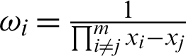is the weight of gravity interpolation.

Using Eq. (2.14), the k derivative of the function at the node can be expressed as

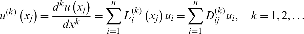
In the form of a matrix as

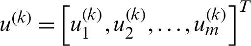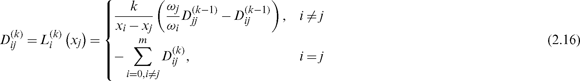
where and are the vector. The matrix is as the k order differential matrix of the function , and 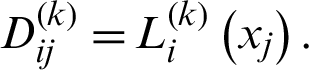In addition, we can calculate (see [25]) with

When the solution of some partial differential equation is obtained by numerical method, it is also necessary to use the differential matrix to calculate the derivative values of the unknown function on calculating nodes.

2.5 Kronecker Product of a Matrix

Kronecker product is an operation form between two matrices of any size and a special form of tensor product. The Kronecker product of any matrix and matrix is recorded as following

where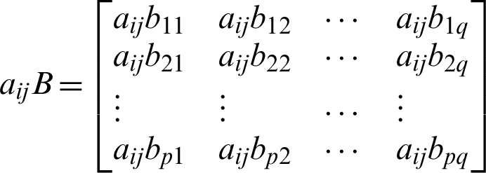

Using the Kronecker product of the barycentric Lagrange interpolation differential matrix, the discrete equation of the Helmholtz equation can be expressed as a simple matrix form.

2.6 Relationship between Partial Derivative of Differential Equation and Differential Matrix

The Kronecker product with the barycentric Lagrange interpolated differential matrix can also be used. The unknown function in the Helmholtz equation has the following corresponding relation between the partial derivative of the variable and the Kronecker product of the corresponding differential matrix.

The number of nodes for the unknown function in x and y directions of the two-dimensional Helmholtz equation are m and n then by using Eq. (2.17), the expressions of the differential matrices corresponding to the partial derivative of the differential equation about the variables x and y can be briefly expressed as

where Im and In represent the unit matrices of m order and n order, respectively, and the and are barycentric interpolates of the second-order matrices at the node and respectively.

Using the above marks, the discrete forms of partial differential equations and boundary conditions can be written directly into matrix form, which makes programming much easier.

3  Discrete Equations of the Two-Dimensional Helmholtz Equation

By substituting the barycenter Lagrange interpolation Eq. (2.9) into Eq. (1.1), we can obtain

If Eq. (3.1) holds at the nodes of , then Eq. (3.1) is replaced by the following

Set . From the properties of the Lagrange interpolation basis, and using Eqs. (2.15), (2.16) and (2.18), then Eq. (3.2) can also be expressed as

Let

Then Eq. (3.3) can be written into

That is

In which .

The above two-dimensional Helmholtz equation is discretized by the barycentric Lagrange interpolation method, and the final scheme is Eq. (3.5). In addition, the boundary conditions need to be discretized, and the following discrete formulas for boundary conditions are elaborated.

By employing Eqs. (2.17) and (2.18), we obtain the matrix form of the boundary condition in Eq. (1.2)

where and represent the first and m lines of the first order differential matrix of the m order unit matrix, and represent the first and n lines of the first order differential matrix of the n order unit matrix, and

Combining Eqs. (3.5) and (3.6), we can obtain the value of the function on each node.

4  Numerical Examples

In this section, we solve some test problems to demonstrate the effectiveness and accuracy of the barycentric Lagrange interpolation method. Six numerical examples of Helmholtz equation including high wavenumber and variable wavenumber problems are given. In which, the maximum absolute error () and relative error ( Er) are defined as follows:

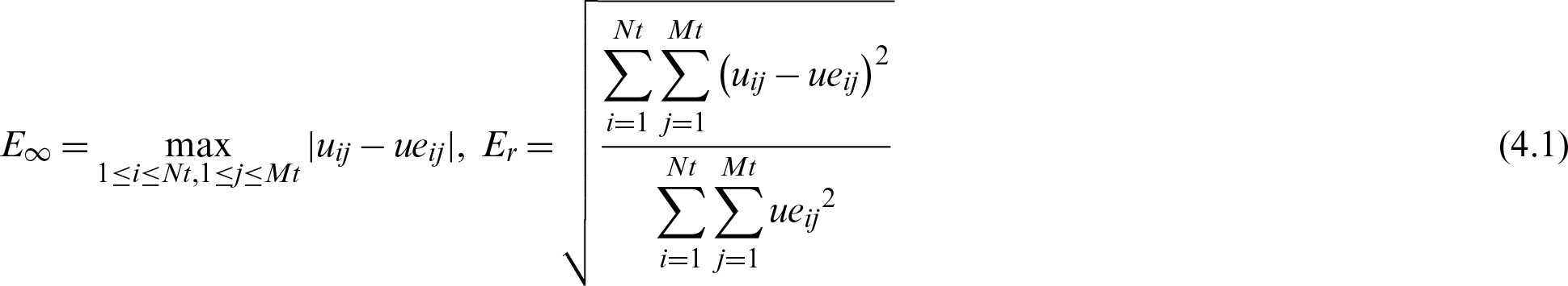
where uij and ueij represent numerical and exact solutions, respectively. Nt and Mt are the numbers of test nodes in the x and y directions, respectively.

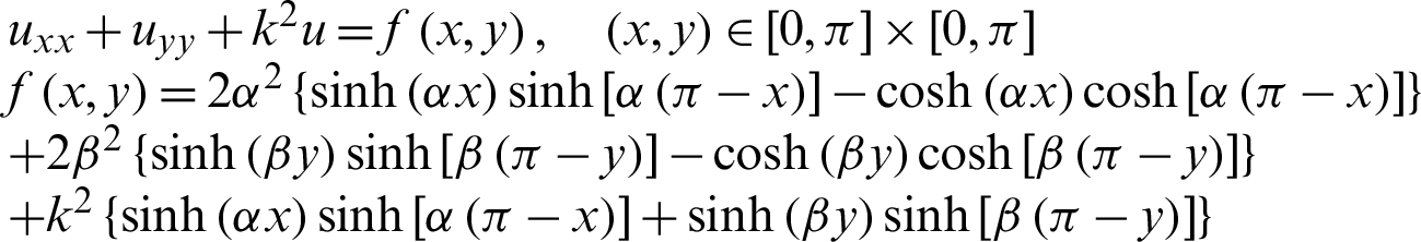
Example 1 [26]:

Consider the following non-homogeneous Helmholtz equation

with the boundary conditions:

The exact solution is

Tab. 1 gives the calculation results of for the four kinds of interpolation nodes with Nt = Mt = N, k = 5. In which, N is the number of interpolation nodes in the domain, Nt and Mt are the numbers of test nodes, and the test nodes type are the second kind of Chebyshev nodes (that is Chebyshev II) rather than the first kind of Chebyshev nodes (that is Chebyshev I). The results show that the random interpolation nodes are bad for our proposed method, the uniform interpolation nodes are not good and the two kinds of Chebyshev interpolation nodes are very good. What’s more, the numerical results show that the accuracy of the Chebyshev node is highest, the stability is best, and the calculation error is smallest. Therefore, we use the two kinds of Chebyshev nodes rather than the random or uniform nodes as the interpolation nodes to calculate the Tabs. 2 and 3 for Example 1. In addition, the numerical results of the Chebyshev II is a little better than that of the Chebyshev I.

Table 1: The with four kinds of interpolation nodes when Nt = Mt = N, k = 5 for Example 1

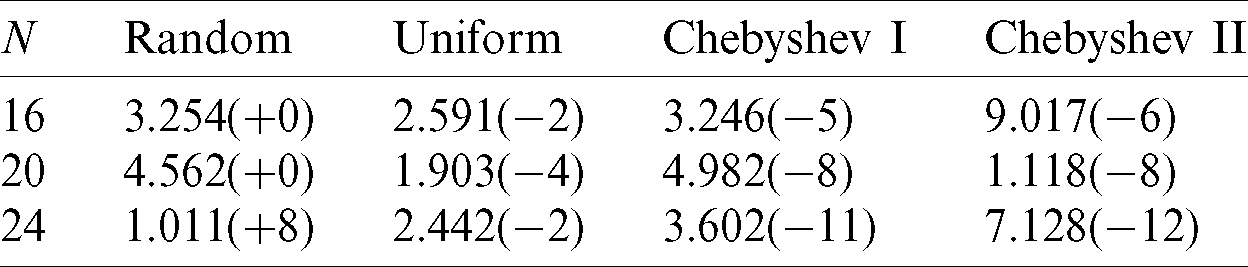
Table 2: The with two kinds of interpolation nodes and three kinds of test nodes when Nt = Mt = 100, k = 5 for Example 1

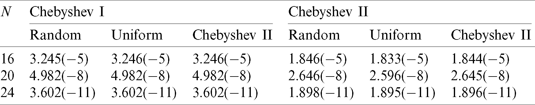
Table 3: The with two kinds of interpolation nodes and three kinds of test nodes when N = 24, k = 5 for Example 1

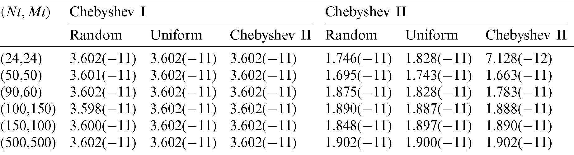
Then the with two kinds of Chebyshev interpolation nodes and three kinds of test nodes when Nt = Mt = 100, k = 5 and N = 24, k = 5 is given in Tabs. 2 and 3, respectively. What should we know is that the two kinds of interpolation nodes here are Chebyshev I and the Chebyshev II. Three kinds of test nodes are random test nodes, uniform test nodes and Chebyshev II test nodes all the time. According to the calculation results, firstly, we can know that the results of Chebyshev II is better than Chebyshev I and there is almost no difference between three kinds of test nodes. In addition, the error, error order and the convergence order is almost constant as Nt and Mt change, which means that the number of test nodes has little influence on our numerical results. So we can take the value of Nt and Mt with any reasonable number in the left numerical examples. What’s more, the numerical results of the Chebyshev II is a little bit better than the Chebyshev I and the convergence order with the two kinds of interpolation nodes is almost identical, therefore, we use the Chebyshev II interpolation nods and three kinds of test nodes to calculate the left numerical examples in our work.

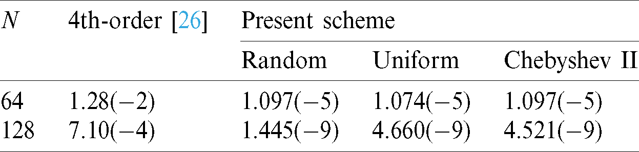
Finally, the calculation results of with the 4th-order method in [26] and with the present scheme are compared when Nt = 130, Mt = 140, k = 30 in Tab. 4. The results show that the error order and the convergence order of the scheme in this paper reaches 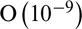and 12th-order, respectively when the number of collocation points is N = 128 , while that in the literature just reaches 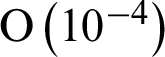and 4th-order, respectively. It shows that the calculation accuracy of the present scheme is much better than that in the literature.

Table 4: The when Nt = 130, Mt = 140, k = 30 for Example 1

The node distribution for the four kinds of interpolation nodes with Nt = Mt = N, k = 5 is shown in Fig. 2. We can observe that the random nodes are distributed randomly within the interval, uniform nodes are distributed equably in the interval and the two kinds of Chebyshev nodes are concentrated at the boundaries while the middle is sparse relatively.

Figure 2: Random (a), uniform (b), Chebyshev I (c) and Chebyshev II (d) interpolation nodes when Nt = Mt = N, k = 5 for Example 1

Then the exact solution with Chebyshev test nodes is plotted in Fig. 3a-III, numerical solutions with random test nodes are plotted in Fig. 3b-I, uniform test nodes in Fig. 3b-II and Chebyshev test nodes in Fig. 3b-III; errors with random test nodes in Fig. 3c-I, uniform test nodes in Fig. 3c-II and Chebyshev test nodes in Fig. 3c-III with Nt = 130, Mt = 140, k = 30, N = 12. Among them, because the exact solutions with three kinds of test nodes are almost the same, we only give the figure with Chebyshev test nodes. In addition, it can be observed that all numerical solutions with the three kinds of test nodes agree well with the exact solution. What’s more, because of the addition of test nodes on the boundaries to calculate the numerical solution with proposed method, these nodes’ values on the boundaries are no longer given by the exact solution and resulting in some error’s appearance on the boundaries. It can also be observed from Fig. 3c that the errors are equivalent with that in the interior region.

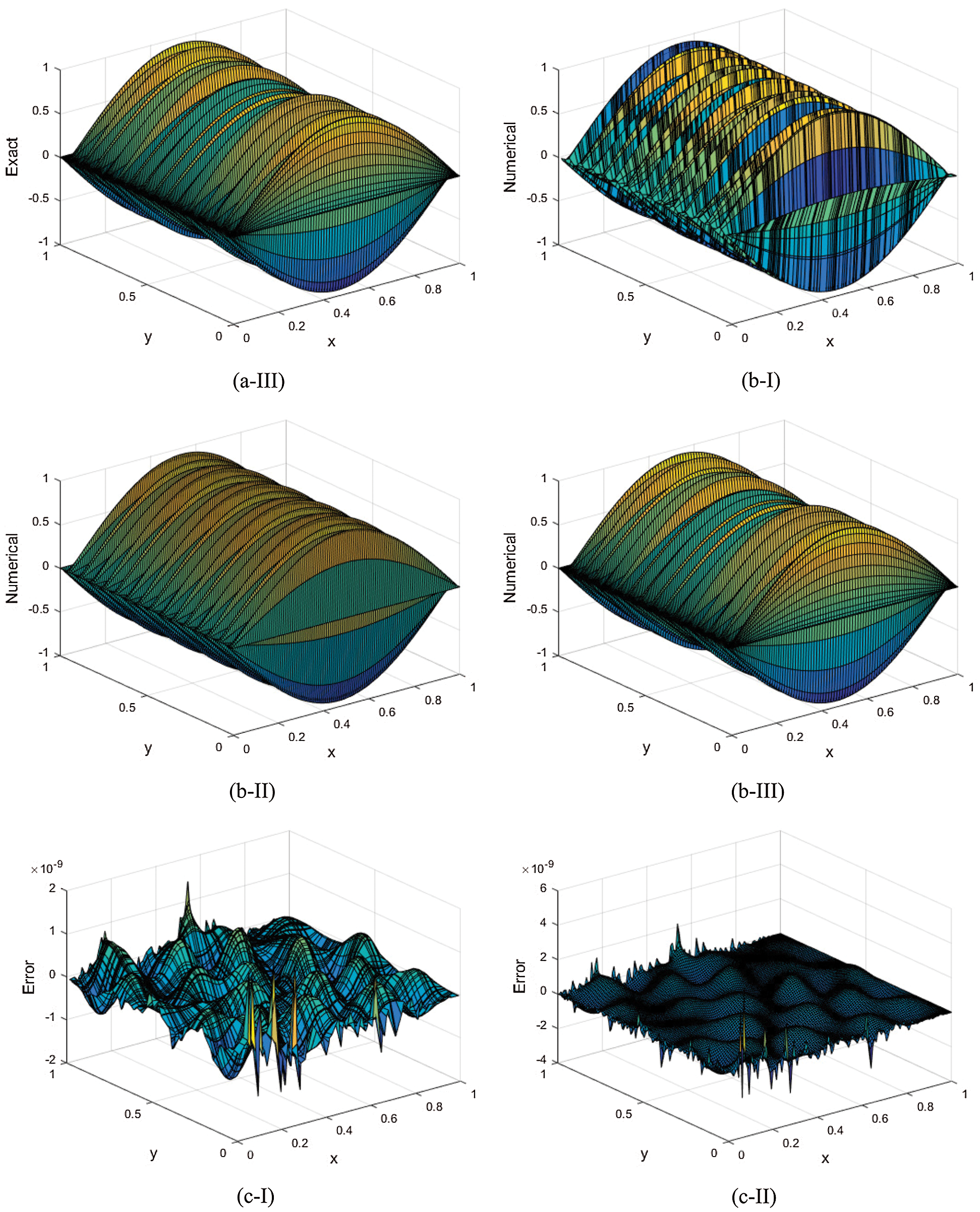
Figure 3: Exact (a) and numerical (b) solutions and error (c) with different test nodes: random (I), uniform (II) and Chebyshev (III) when Nt = 130, Mt = 140, k = 30, N = 128 for Example 1

Finally, the convergence order with Nt = Mt = 100, k = 5 and Nt = 130, Mt = 140, k = 30 is shown in Fig. 4. It can be seen that with the wave number of k increases, the order of convergence decreases. Meanwhile, the convergence order of the two kinds of interpolation nodes Chebyshev I and Chebyshev II is almost identical. And then the convergence order of the proposed method is much higher than that in the literature.

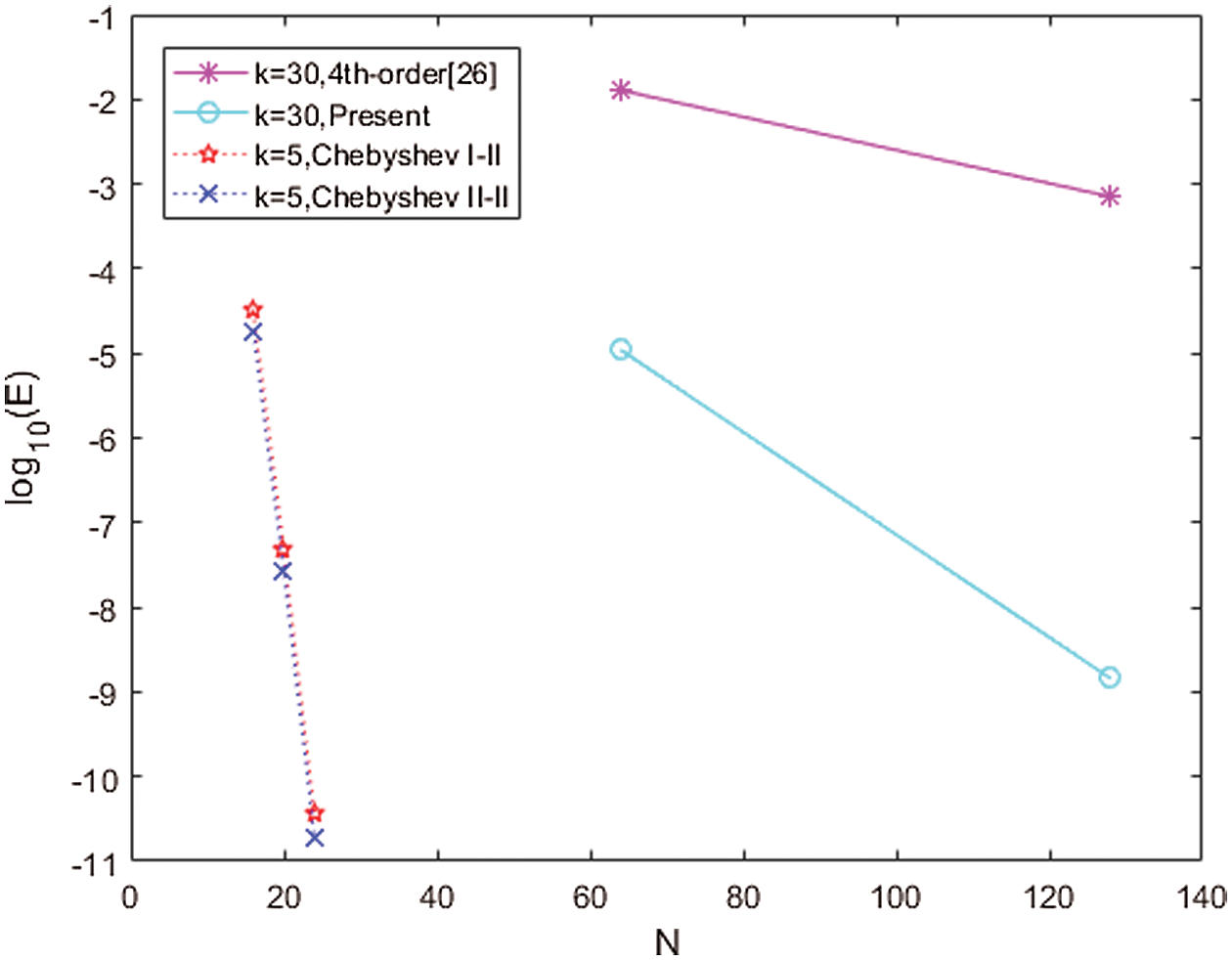
Figure 4: The convergence order with Nt = Mt = 100, k = 5 and Nt = 130, Mt = 140, k = 30 for Example 1

Example 2 [27]:

Consider the following non-homogeneous Helmholtz equation

with the boundary conditions:

The exact solution is

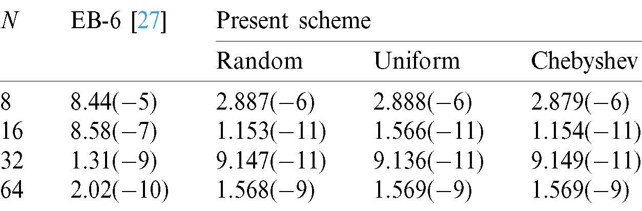
Tab. 5 gives the computed by the present scheme and compares with EB-6 method in [27] when . The results show that the error order of the proposed scheme reaches when the number of collocation points is N = 16 , while that in the literature, the error order only reaches when N = 16 and when N = 64. Therefore, the number of calculation points needed in the present scheme is much less than that in the literature and we can save more computational amount. In addition, we notice the error order of the proposed scheme decreases gradually and the error increase gradually with the increase of the number of nodes N , but the overall calculation result is better than that in the literature. What’s more, convergence order of the proposed method is the 21th-order, while that in the literature is the 6th-order, so the precision of present method is also better than the method in the literature. Compared with the finite difference method, the barycentric Lagrange interpolation collocation method does not mean that the more nodes there are, the better the calculation results will be. Sometimes, we can obtain the better results with comparably a few nodes.

Table 5: The when for Example 2

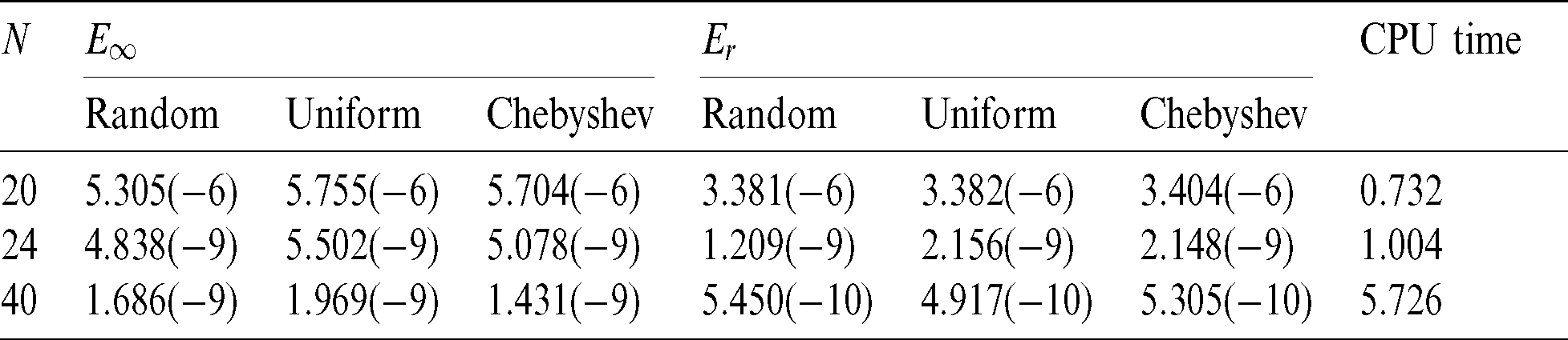
The and CPU time with are given in Tab. 6. It shows that the proposed scheme can approximate the exact solution with a few nodes. It is necessary to note that for the determination of CPU time in our work, we select the longest time taken by the three test nodes method. Even so, we still find that for the two-dimensional Helmholtz equation, the CPU time with the present scheme is very small when the number of collocation points is less, which shows that this method is less time-consuming and can save calculation time effectively.

Table 6: The 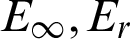and CPU time when for Example 2

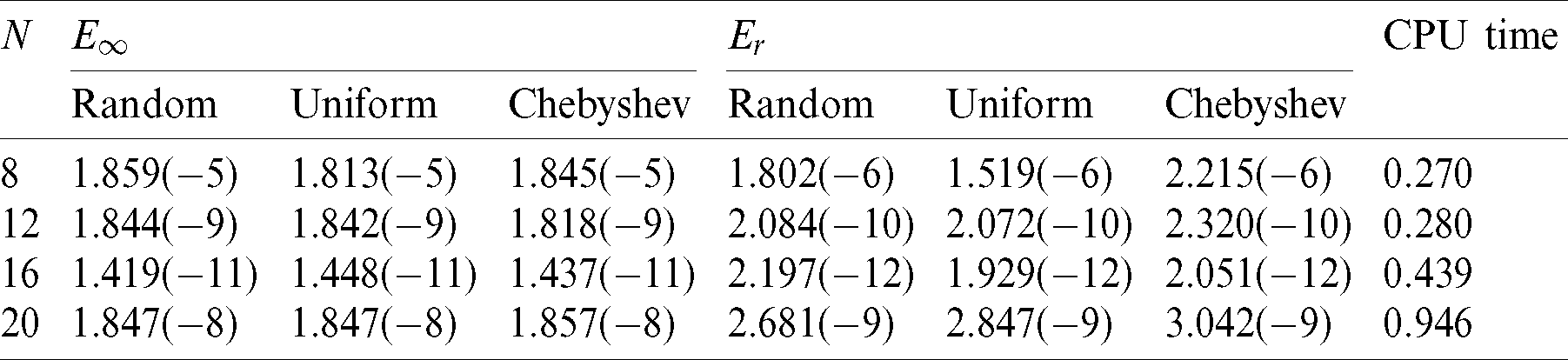
Fig. 5. gives the exact (a) and numerical (b) solutions and error (c) with different test nodes: random (I), uniform (II) and Chebyshev (III) with It shows that the numerical solution with three kinds of test nodes have the similar shape and are in good agreement with the exact solution as well. What’s more, Figs. 3c-I, 3c-II and 3c-III show that the error order reaches .

Figure 5: Exact (a) and numerical (b) solutions and error (c) with different test nodes: random (I), uniform (II) and Chebyshev (III) when for Example 2

Example 3 [28]:

Consider the following non-homogeneous high wavenumber Helmholtz equation

with the boundary conditions:

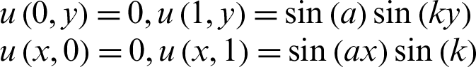
The exact solution is

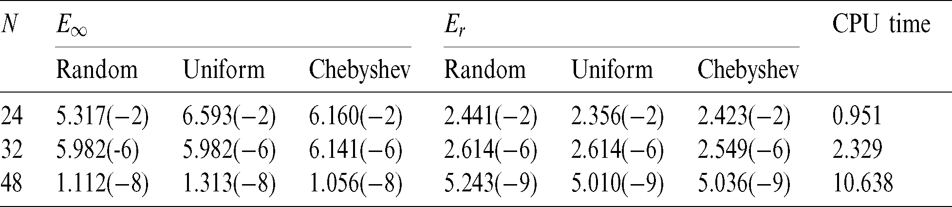
The calculation results with the 6th-order method in [28] and the present scheme are compared under different wave numbers with k = 24 and k = 48 when a = 1, Nt = 130, Mt = 150 in Tab. 7. The results show that the calculation error and error order of the present scheme are much better than that in the literature. Therefore, it is more suitable for solving high wavenumber problems as well. Then the and CPU time with a = 0.5, Nt = Mt = 60, k = 12 are given in Tab. 8. It shows the advantages of the present scheme, such as less number of collocation points, short calculation time, high precision and small error.

Table 7: The with different wave numbers when a = 1, Nt = 130, Mt = 150 for Example 3

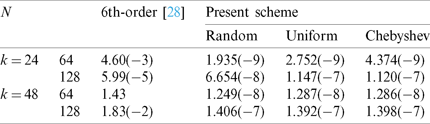
Table 8: The and CPU time when a = 0.5, Nt = Mt = 60, k = 12 for Example 3

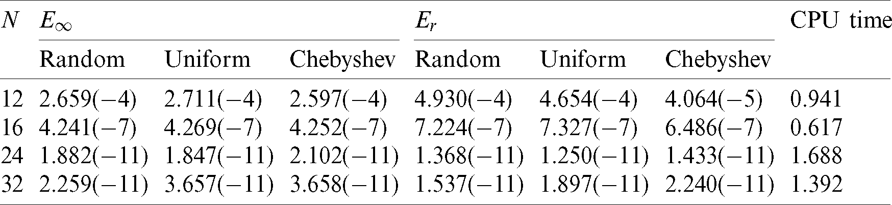
Fig. 6. gives the exact (a) and numerical (b) solutions and error (c) with different test nodes: random (I), uniform (II) and Chebyshev (III) with a = 1, Nt = 130, Mt = 150, k = 48, N = 128, respectively. It shows that the numerical solutions agree very well with the exact solution, and the error of three kinds of test nodes has little difference.

Figure 6: Exact (a) and numerical (b) solutions and error (c) with different test nodes: random (I), uniform (II) and Chebyshev (III) when a = 1, Nt = 130, Mt = 150, k = 48, N = 128 for Example 3

Example 4 [29]:

Consider the following non-homogeneous variable wavenumber Helmholtz equation

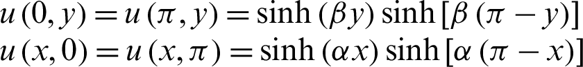
with the boundary conditions:

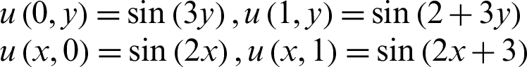
The exact solution is

Tab. 9 shows the when Nt = 150, Mt = 130 with variable wavenumber . Compared with the MHADI method in [29], the error order of the present scheme is with N = 16 , while that in the literature is only . In addition, the accuracy in the literature is the 4th-order, while that in this paper is up to the 9th-order. So the present scheme has higher calculation accuracy compared with that in the literature. We notice that although the error order of the proposed scheme decreases with the increase of the number of nodes, the overall calculation results are still better than that in the literature. Then the at different collocation points and CPU time with Nt = Mt = 50, are given in Tab. 10. The numerical results show that compared with the finite difference, the barycentric Lagrange interpolation method is more suitable for solving the problem of variable wavenumber. At the same time, we can obtain the better results with relatively a few nodes.

Table 9: The when for Example 4

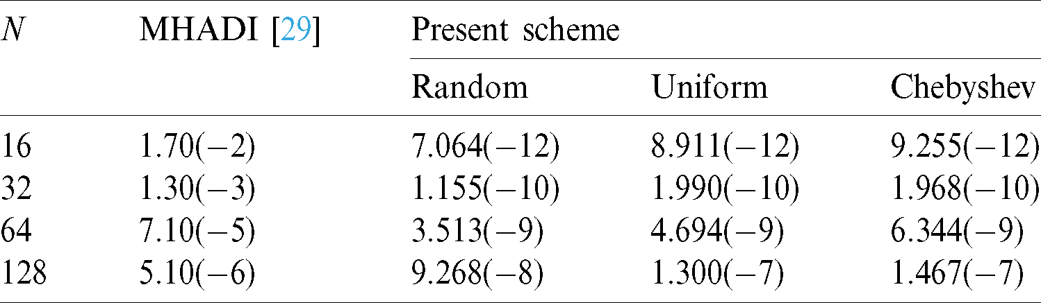
Table 10: The and CPU time when for Example 4

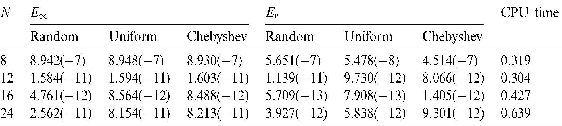
Fig. 7. gives the exact (a) and numerical (b) solutions and error (c) with different test nodes: random (I), uniform (II) and Chebyshev (III) with respectively. It shows that although k is the variable wavenumber, the numerical solutions are also in good agreement with the exact solution, and the error is steady as a whole.

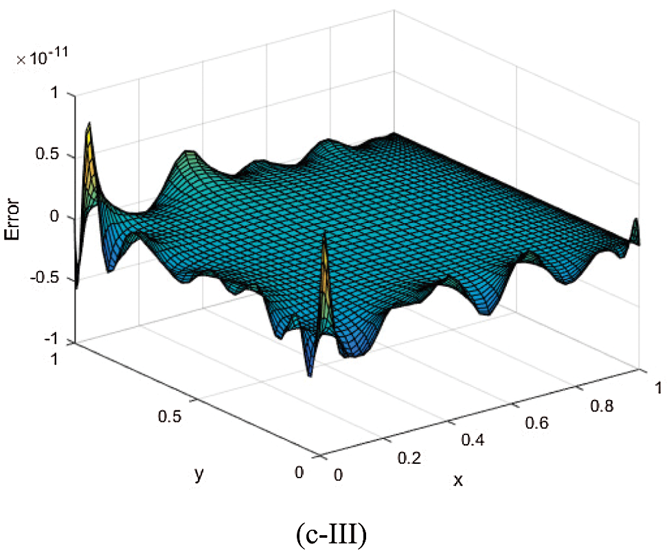
Figure 7: Exact (a) and numerical (b) solutions and error (c) with different test nodes: random (I), uniform (II) and Chebyshev (III) when for Example 4

Table 12: The and CPU time when Nt = Mt = 50, k = 10 for Example 5

Example 5 [30]:

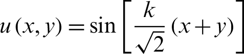
Consider the following homogeneous Helmholtz equation

with the Dirichlet boundary condition. The computational domain is an ameba-shape domain (see Fig. 7) with the boundary defined by the parametric equation:

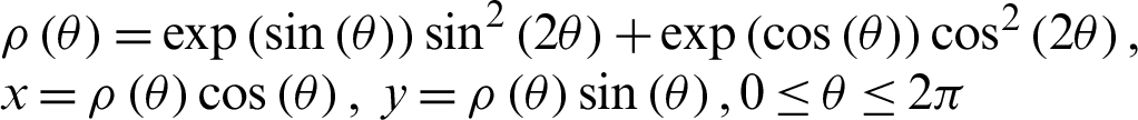
The exact solution is

Tab. 11 and Tab. 12 give the and CPU time with an ameba-shape domain when Nt = Mt = 50, k = 5 and Nt = Mt = 50, k = 10, respectively. What should be noted is that the [30] only computed a square domain, so we do not make comparisons with it and just give the results of our proposed method. The results show that even in an arbitrary region, the accuracy and convergence order of the present method are still very high. It is obvious that the present method is an effective method with high precision.

Table 11: The and CPU time when Nt = Mt = 50, k = 5 for Example 5

Then the Fig. 8. gives the computational domain with different test nodes: random (a), uniform (b) and Chebyshev (c) when Nt = Mt = 50, k = 10, N = 48. Similar to Fig. 1, we can observe the distribution of the three test nodes. Fig. 9. gives the exact (a) and numerical (b) solutions and error (c) with different test nodes: random (I), uniform (II) and Chebyshev (III) with Nt = Mt = 50, k = 10, N = 48. It shows that the even though under the general domain, the numerical solutions agree very well with the exact solution, and the errors of three kinds of test nodes have little difference.

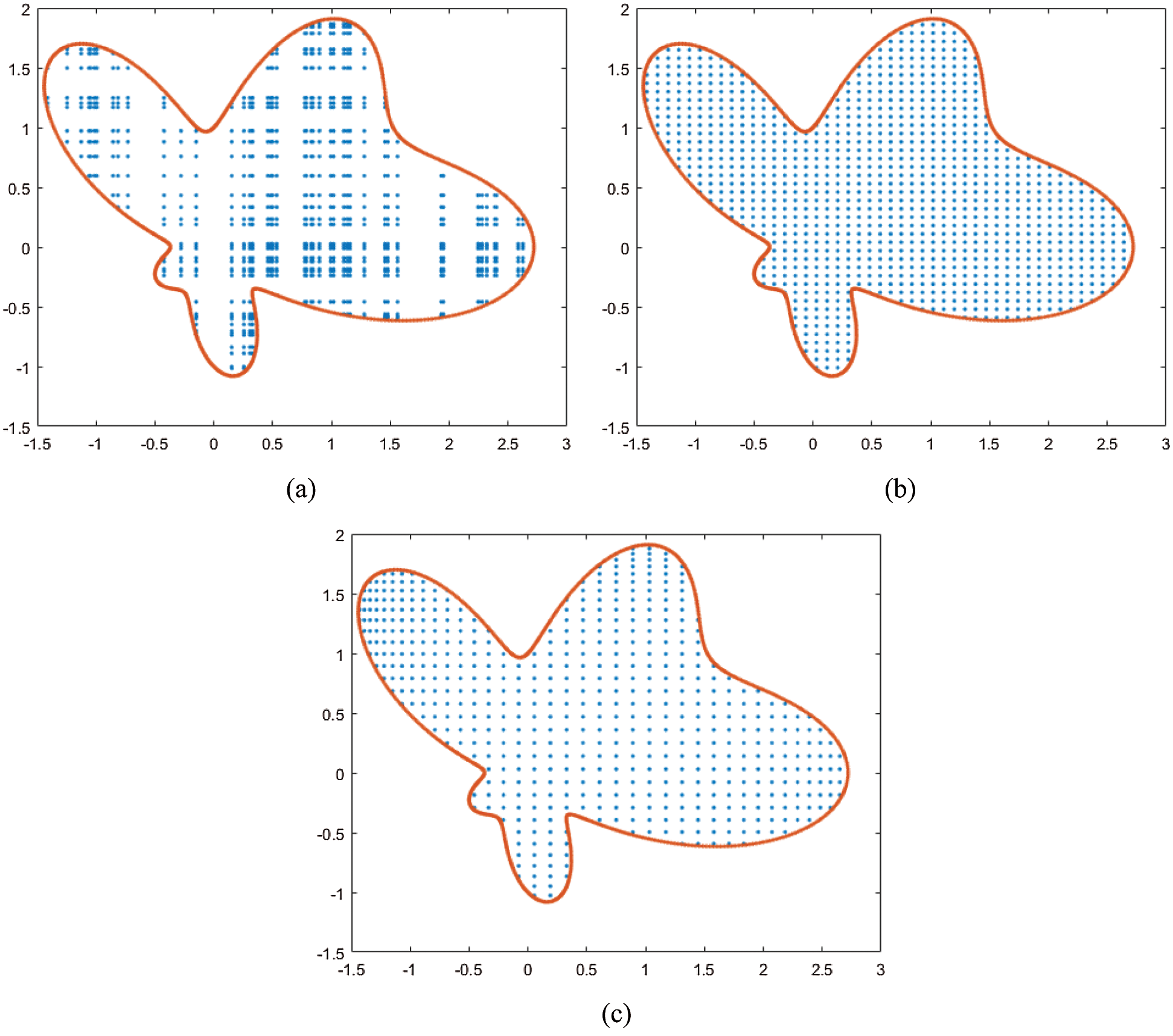
Figure 8: The ameba-shape domain with different test nodes: random (a), uniform (b) and Chebyshev (c) when Nt = Mt = 50, k = 10, N = 48 for Example 5

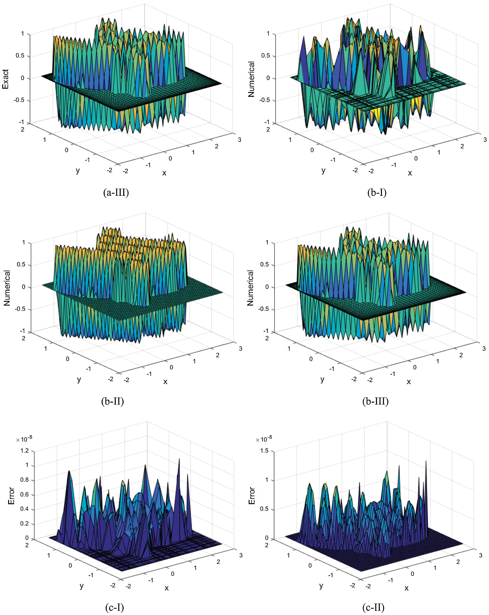
Figure 9: Exact (a) and numerical (b) solutions and error (c) with different test nodes: random (I), uniform (II) and Chebyshev (III) when Nt = Mt = 50, k = 10, N = 48 for Example 5

Example 6 [30]:

Consider the following non-homogeneous modified Helmholtz equation

with the boundary conditions:

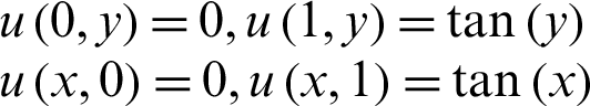
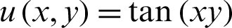
The exact solution is

Lastly, we consider the non-homogeneous modified Helmholtz equation for Example 6. Tab. 13 gives calculation results with the present scheme and compared with [30]. Then the and CPU time with different collocation points under Nt = Mt = 50 is given in Tab. 14. We find that the error and convergence order of our proposed method are still much better than that in the literature. Fig. 10 gives the exact (a), numerical (b) solutions and error (c) with different test nodes: random (I), uniform (II) and Chebyshev (III) when Nt = Mt = 50, N = 16 for Example 6. It is interesting that the proposed scheme is also suitable for non-homogeneous modified Helmholtz equation, and the numerical solution and the exact solution are in good agreement as well, at the same time the error is stable as a whole.

Table 13: The when Nt = Mt = 50 for Example 6

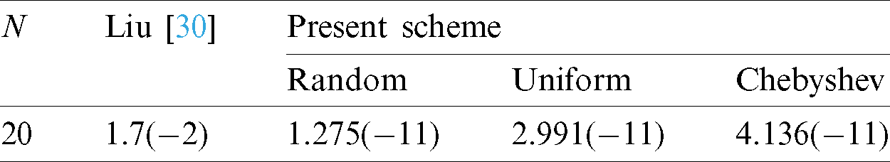
Table 14: The and CPU time when Nt = Mt = 50 for Example 6

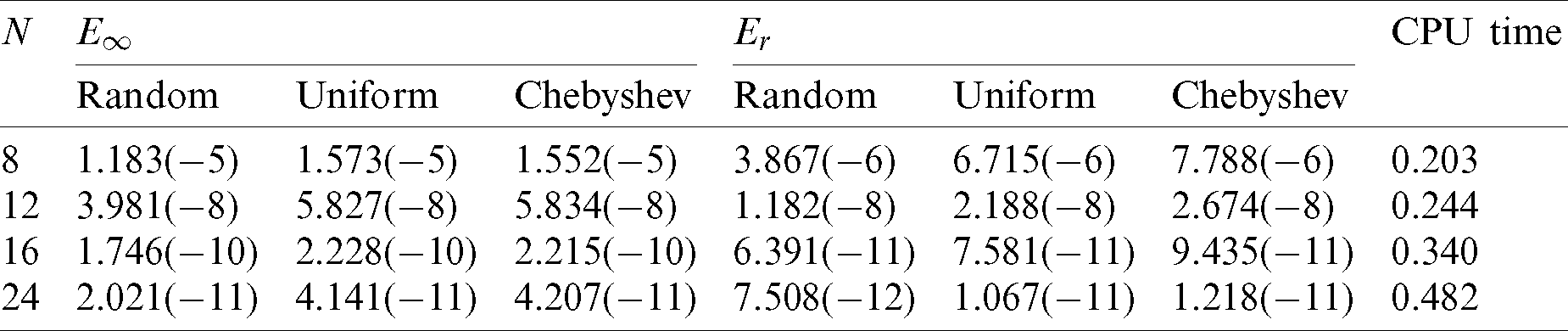
Figure 10: Exact (a) and numerical (b) solutions and error (c) with different test nodes: random (I), uniform (II) and Chebyshev (III) when Nt = Mt = 50, N = 16 for Example 6

5  Conclusions

Based on the Chebyshev interpolation nodes, we have developed a meshless collocation method for solving the two-dimensional Helmholtz equations with the Dirichlet boundary condition, by using the barycentric Lagrange interpolation basis function. Firstly, this meshless collocation method applies the interpolation basis function to treat the spatial variables and their partial derivatives, and establishes the collocation method for solving the differential equations. Secondly, at a given node, the multivariate basis function is substituted into the equation and its boundaries and the discrete algebraic equations are obtained. Then, the differential matrix is used to simplify it. To investigate the accuracy and efficiency of the proposed method, we conduct some numerical experiments by using three kinds of test nodes. Based on our research, we can draw some conclusions as follows:

1.    As for the choice of interpolation nodes, the numerical results show that Chebyshev II is better than Chebyshev I for the present scheme. As for test nodes, there is almost no difference for the numerical results with three kinds of test nodes. In addition, with the change of the number of test nodes Nt and Mt, the error is almost unchanged. That is say that the number of test nodes has little influence for the numerical results.

2.    By using comparably fewer nodes, the present scheme can obtain high-precision numerical results and keep good stability compared with those methods in the literature. It shows the advantages of the present scheme, such as smaller number of collocation points needed, short calculation time, high precision, small error and high efficiency. What’s more, the numerical solutions agree well with the exact solutions.

3.    Compared with the methods in the literature, the present method can not only calculate the high wavenumber problems, but also calculate the variable wavenumber problems, and the numerical results are better than those in the literature. For modified Helmholtz equation, the results computed by the present scheme are far better than those in the literature as well.

4.    The present method can be extended to solve the 3D Helmholtz equations. We will report it in the near future.

Funding Statement: The authors would like to thank very mush to the anonymous reviewers whose constructive comments are helpful for this paper’s revision. This work is partially supported by National Natural Science Foundation of China (11772165, 11961054, 11902170), Key Research and Development Program of Ningxia (2018BEE03007), National Natural Science Foundation of Ningxia (2018AAC02003, 2020AAC03059), and Major Innovation Projects for Building First-class Universities in China’s Western Region (Grant No. ZKZD2017009).

Conflicts of Interest: The authors declare that they have no conflicts of interest to report regarding the present study.

References

 1.  Assari, P., Fatemeh, A., Cuomo, M. S. (2019). A numerical scheme for solving a class of logarithmic integral equations arisen from two-dimensional Helmholtz equations using local thin plate splines. Applied Mathematics and Computation, 356, 157–172. DOI 10.1016/j.amc.2019.03.042. [Google Scholar] [CrossRef]

 2.  Wang, K. Y., Wang, Q. S. (2013). Study on vibration of membranes with Taylor polynomial method and error analysis for Helmholtz equation. Advanced Materials Research, 763, 234–237. DOI 10.4028/www.scientific.net/AMR.763.234. [Google Scholar] [CrossRef]

 3.  Jo, C. H., Shin, C., Suh, J. H. (1996). An optimal 9-point, finite-difference, frequency-space, 2-D scalar wave extrapolato. Geophysics, 61(2), 529–537. DOI 10.1190/1.1443979.

 4.  Du, K. (2011). A composite preconditioner for the electromagnetic scattering from a large cavity. Journal of Computational Physics, 230(22), 8089–8108. DOI 10.1016/j.jcp.2011.07.011.

 5.  Wang, S., Hoop, M. V. D., Xia, J. L. (2010). Acoustic inverse scattering via Helmholtz operator factorization and optimization. Journal of Computational Physics, 229(22), 8445–8462. DOI 10.1016/j.jcp.2010.07.027.

 6.  Liu, G., Jayathilake, P. G., Khoo, B. C., Han, F., Liu, D. K. (2012). Conformal mapping for the Helmholtz equation: Acoustic wave scattering by a two dimensional inclusion with irregular shape in an ideal fluid. Journal of the Acoustical Society of America, 131(2), 1055–1065. DOI 10.1121/1.3675947. [Google Scholar] [CrossRef]

 7.  Linton, C. M. (2010). Lattice sums for the Helmholtz equation. SIAM Review, 52(4), 630–674. DOI 10.1137/09075130X. [Google Scholar] [CrossRef]

 8.  Swager, M. R., Gray, L. J., Fata, S. N. (2010). Galerkin boundary integral analysis for the 3D Helmholtz equation. Computer Modeling in Engineering & Sciences, 58(3), 297–234. [Google Scholar]

 9.  Tsai, C. C., Young, D. L. (2013). Using the method of fundamental solutions for obtaining exponentially convergent Helmholtz eigensolutions. Computer Modeling in Engineering & Sciences, 94(1), 175–205. [Google Scholar]

10. Wu, T. T. (2017). A dispersion minimizing compact finite difference scheme for the 2D Helmholtz equation. Journal of Computational and Applied Mathematics, 311, 497–512. DOI 10.1016/j.cam.2016.08.018. [Google Scholar] [CrossRef]

11. Liu, G. R., Gu, Y. T. (2005). An introduction to meshfree method and their programming, Berlin, New York: Springer. [Google Scholar]

12. Reutskiy, S. Y. (2006). The method of external sources (MES) for eigenvalue problems with Helmholtz equation. Computer Modeling in Engineering & Sciences, 12(1), 27–39. [Google Scholar]

13. Chen, H. X., Qiu, W. F. (2017). A first order system least squares method for the Helmholtz equation. Journal of Computational and Applied Mathematics, 309, 145–162. DOI 10.1016/j.cam.2016.06.019. [Google Scholar] [CrossRef]

14. Dogan, H., Popov, V., Ooi, E. H. (2015). Dispersion analysis of the meshless local boundary integral equation and radial basis integral equation methods for the Helmholtz equation. Engineering Analysis with Boundary Elements, 50, 360–371. DOI 10.1016/j.enganabound.2014.09.009. [Google Scholar] [CrossRef]

15. Chen, L. C., Li, X. L. (2020). A Burton–Miller boundary element-free method for Helmholtz problems. Applied Mathematical Modelling, 83, 386–399. DOI 10.1016/j.apm.2020.03.009. [Google Scholar] [CrossRef]

16. Qu, W. Z., Fan, C. M., Gu, Y. (2019). Localized method of fundamental solutions for interior Helmholtz problems with high wave number. Engineering Analysis with Boundary Elements, 107, 25–32. DOI 10.1016/j.enganabound.2019.06.018. [Google Scholar] [CrossRef]

17. Britt, S., Petropavlovsky, S., Tsynkov, S., Turkel, E. (2015). Computation of singular solutions to the Helmholtz equation with high order accuracy. Applied Numerical Mathematics, 93, 215–241. DOI 10.1016/j.apnum.2014.10.006. [Google Scholar] [CrossRef]

18. Lin, J., Chen, W., Chen, C. S., Jiang, X. R. (2020). Fast bundary knot method for solving axisymmetric Helmholtz problem with high wave number. Computer Modeling in Engineering & Sciences, 94(6), 485–505. [Google Scholar]

19. Wang, K., Wong, Y. S., Huang, J. Z. (2017). Solving Helmholtz equation at high wave numbers in exterior domains. Applied Mathematics and Computation, 298, 221–235. DOI 10.1016/j.amc.2016.11.015. [Google Scholar] [CrossRef]

20. Li, X. L., Dong, H. Y. (2020). Error analysis of the meshless finite point method. Applied Mathematics and Computation, 382, 125326. DOI 10.1016/j.amc.2020.125326. [Google Scholar] [CrossRef]

21. Qu, W. Z., Fan, C. M., Li, X. L. (2020). Analysis of an augmented moving least squares approximation and the associated localized method of fundamental solutions. Computers and Mathematics with Applications, 80(1), 13–30. DOI 10.1016/j.camwa.2020.02.015. [Google Scholar] [CrossRef]

22. Berrut, J. P., Trefethen, L. N. (2004). Baryccentric lagrange interpolation. SIAM Review, 46(3), 501–517. DOI 10.1137/S0036144502417715. [Google Scholar] [CrossRef]

23. Ma, W. T., Zhang, B. W., Ma, H. L. (2016). A meshless collocation approach with barycentric rational interpolation for two-dimensional hyperbolic telegraph equation. Applied Mathematics and Computation, 279, 236–248. DOI 10.1016/j.amc.2016.01.022. [Google Scholar] [CrossRef]

24. Kumar, S. (2014). A new analytical modeling for fractional telegraph equation via Laplace transform. Applied Mathematical Modelling, 38(13), 3154–3163. DOI 10.1016/j.apm.2013.11.035. [Google Scholar] [CrossRef]

25. Berrut, J. P., Baltensperger, R., Mittelmann, H. D. (2005). Recent developments in barycentric rational interpolation. International Series of Numerical Mathematics, 151, 27–51. [Google Scholar]

26. Fu, Y. P. (2008). Compact fourth-order finite difference schemes for Helmholtz equation with high wave numbers. Journal of Computational Mathematics, 26, 98–111. [Google Scholar]

27. Singer, I., Turkel, E. (2006). Sixth-order accurate finite difference schemes for the Helmholtz equation. Journal of Computational Acoustics, 214(03), 339–351. DOI 10.1142/S0218396X06003050. [Google Scholar] [CrossRef]

28. Wu, T. T., Xu, R. M. (2018). An optimal compact sixth-order finite difference scheme for the Helmholtz equation. Computers and Mathematics with Applications, 75(7), 2520–2537. DOI 10.1016/j.camwa.2017.12.023. [Google Scholar] [CrossRef]

29. Zhuang, Y., Sun, X. H. (2000). A high order ADI method for separable generalized Helmholtz equations. Advances in Engineering Software, 31(8–9), 585–591. DOI 10.1016/S0965-9978(00)00026-0. [Google Scholar] [CrossRef]

30. Liu, C. S., Kuo, C. L. (2016). A multiple-scale Pascal polynomial triangle solving elliptic equations and inverse Cauchy problems. Engineering Analysis with Boundary Elements, 62, 35–43. DOI 10.1016/j.enganabound.2015.09.003. [Google Scholar] [CrossRef]

This work is licensed under a Creative Commons Attribution 4.0 International License, which permits unrestricted use, distribution, and reproduction in any medium, provided the original work is properly cited.