| Computer Modeling in Engineering & Sciences |
DOI: 10.32604/cmes.2021.012218
ARTICLE
A Novel BEM for Modeling and Simulation of 3T Nonlinear Generalized Anisotropic Micropolar-Thermoelasticity Theory with Memory Dependent Derivative
1 Jamoum University College, Umm Al-Qura University, Makkah, Saudi Arabia
2Faculty of Computers and Informatics, Suez Canal University New Campus, Ismailia, 41522, Egypt
*Corresponding Author: Mohamed Abdelsabour Fahmy. Email: maselim@uqu.edu.sa; mohamed_fahmy@ci.suez.edu.eg
Received: 20 June 2020; Accepted: 10 September 2020
Abstract: The main aim of this paper is to propose a new memory dependent derivative (MDD) theory which called three-temperature nonlinear generalized anisotropic micropolar-thermoelasticity. The system of governing equations of the problems associated with the proposed theory is extremely difficult or impossible to solve analytically due to nonlinearity, MDD diffusion, multi-variable nature, multi-stage processing and anisotropic properties of the considered material. Therefore, we propose a novel boundary element method (BEM) formulation for modeling and simulation of such system. The computational performance of the proposed technique has been investigated. The numerical results illustrate the effects of time delays and kernel functions on the nonlinear three-temperature and nonlinear displacement components. The numerical results also demonstrate the validity, efficiency and accuracy of the proposed methodology. The findings and solutions of this study contribute to the further development of industrial applications and devices typically include micropolar-thermoelastic materials.
Keywords: Boundary element method; memory dependent derivative; three-temperature; nonlinear generalized anisotropic micropolar-thermoelasticity
The study of thermoelastic models has recently gained growing attention due to its many applications in aerospace technologies, geophysics, aeronautics, astronautics, robotics, earthquake engineering, mining engineering, nuclear energy industry, military technologies, soil dynamics, high-energy particle accelerators and detectors, and other engineering and electronic industries [1–9].
The classical thermo-elasticity (CTE) theory of Duhamel [10] and Newman [11] has two deficiencies: the first deficiency is the heat conduction of CTE does not include any elastic term, whereas the second deficiency is that, the equation of heat conduction has infinite heat propagation velocities. In order to overcome the first deficiency, Biot [12] proposed classical coupled thermo-elasticity (CCTE). But CTE and CCTE have the second deficiency. Therefore, many generalized thermo-elasticity theories have been developed to overcome the second deficiency of CTE. Among these theories are extended thermo-elasticity (ETE) theory of Lord et al. [13], temperature-rate-dependent thermo-elasticity (TRDTE) theory of Green et al. [14–16] namely I, II and III, respectively, (where, GN theory I is based on Fourier’s law of heat conduction and identical to CTE theory, GN theory II characterizes the thermoelasticity without energy dissipation (TEWOED), and GN theory III which characterizes the thermoelasticity with energy dissipation (TEWED)). Although most thermal phenomena are practically represented using the classical Fourier thermal conductivity equation [17–22], there are a large number of applications that require the use of the nonlinear heat conduction equation, great attention has been paid to investigate of nonlinear generalized thermoelastic problems by using boundary element method [23–26]. Fahmy [27] introduced the three-temperature theory in the context of nonlinear generalized thermoelasticity.
The fractional calculus is the mathematical branch that is used to study the theory and applications of derivatives and integrals of arbitrary non-integer order. Recently, this branch has emerged as an effective tool for modeling of various engineering and industrial applications [28,29]. Due to the nonlocal nature of fractional order operators, they are useful for describing the memory and hereditary properties of various materials and processes. Also, the fractional calculus has drawn wide attention from the researchers of various countries in recent years due to its applications in solid mechanics, fluid dynamics, quantum mechanics, viscoelasticity, heat conduction modeling and identification, biology, food engineering, econophysics, biophysics, biochemistry, electrochemistry, electrical engineering, finance and control theory, robotics and control theory, signal and image processing, electronics, electric circuits, wave propagation, nanotechnology, flabby, oscillation, stochastic diffusion theory and wave propagation, etc. [30–32].
Several famous mathematicians have contributed to the development of fractional order calculus, where Euler mentioned interpolating between integral orders of a derivative in 1730. At that point, Laplace characterized a fractional derivative by implies of an integral in 1812.
Lacroix presented the first formula for the fractional order derivative appeared in 1819, where he introduced the  th derivative of the function
  as follows

In 1967, the Italian mathematician Caputo presented his fractional derivative of order  as
as

Diethelm [33] has suggested the derivative of Caputo in the form below

where  is the
  -th order derivative and
  is an integer such that

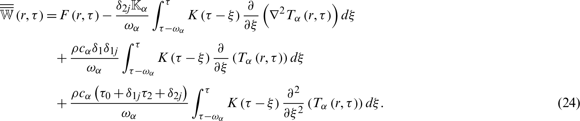
Wang et al. [34] have introduced MDD as follows

where the first order ( ) of MDD for a differentiable function
  can be expressed as

Based on several practical applications, the memory effect needs weight  for
for  , so the MDD magnitude
  is usually smaller than
  , where the kernel function (
 for
for  ) Can be randomly selected over a staggered interval
  , the practical kernel functions are 1,
  and
and  ,
, 
 , 1, 2, etc. These functions are monotonically increasing with
  for the past time
  and
and  for the present time
  . The main feature of MDD, that the real-time functional value depends also, on the past time
  . So,
. So,  depends on the past time (nonlocal operator), while the integration doesn’t depend on the past time (local operator).
As a special case  we have

The above equation shows that the common derivative  is the limit of
  as
as  . That is,

Due to the computational difficulties in solving nonlinear generalized anisotropic thermoelastic problems, the problems become too complicated with no general analytical solution. So, numerical solutions should be implemented instead of analytical solutions to obtain the approximate solutions for such problems, one of the best of these numerical methods is the boundary element method (BEM) [35,36], which also called boundary integral equation method. BEM has been extensively used for a large variety of engineering and industrial applications. In the BEM, only the boundary of the computational domain needs to be discretized, so, it has a major advantage over domain methods which requires the whole computational domain discretization such as the finite difference method (FDM) [37–39] and finite element method (FEM) [40–42]. This advantage of BEM over domain methods has significant importance for modeling of nonlinear generalized thermoelastic problems which can be implemented using BEM with little cost and less input data [43–57]. Through this paper, we would like to guide the reader to this important paper of Cheng et al. [58] which narrates BEM history in a wonderful and interesting way. Sladek et al. [59–61] and Huang et al. [62] developed the boundary element formulation for micropolar thermoelasticity.
Researchers in numerical methods were only aware of the importance of FEM which could solve complex engineering problems. But now after the huge achievements of BEM and their ability to solve inhomogeneous and non-linear problems involving infinite and semi-infinite domains very efficiently, they realized the power, ease and accuracy of BEM in solving their complex problems by using a lot of software like FastBEM and BEASY.
The main aim of this paper is to propose a new MDD theory, called three-temperature nonlinear generalized anisotropic micropolar-thermoelasticity and propose a novel BEM technique for solving problems associated with the proposed theory. The numerical findings are graphically represented to demonstrate the impacts of the time delays and kernel functions on the total nonlinear three-temperature and nonlinear displacement components and demonstrate the validity and exactness of the suggested technique.
A brief summary of this paper is as follows: Section 1 introduces the background and provides the readers with the necessary information to books and articles for a better understanding of thermoelasticity theories, memory dependent derivative history and their applications. Section 2 describes the physical modeling of memory dependent derivative problems of three-temperature nonlinear generalized anisotropic micropolar-thermoelasticity. Section 3 outlines the BEM implementation for obtaining the temperature field of the considered problem. Section 4 outlines the BEM implementation for obtaining the displacement field of the considered problem. Section 5 introduces the computational performance of the proposed technique. Section 6 presents the new numerical results that describe the effects of time delays and kernel functions on the total temperature and displacement components. Section 7 outlines the significant findings of this paper.
The geometry of the considered problem is shown in Fig. 1 for a structure which occupies the bounded region 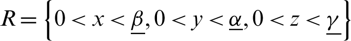 that bounded by S, where Si
  such that S1 +S2 = S3 +S4 = S.
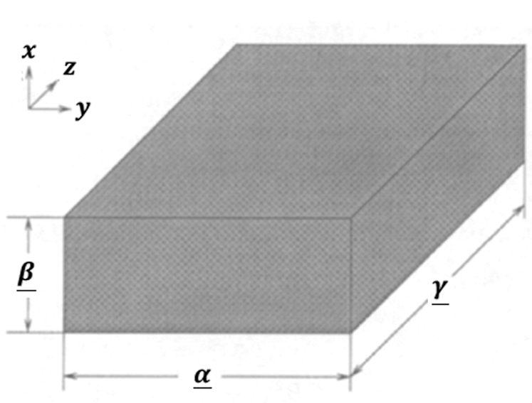
Figure 1: Geometry of the considered problem
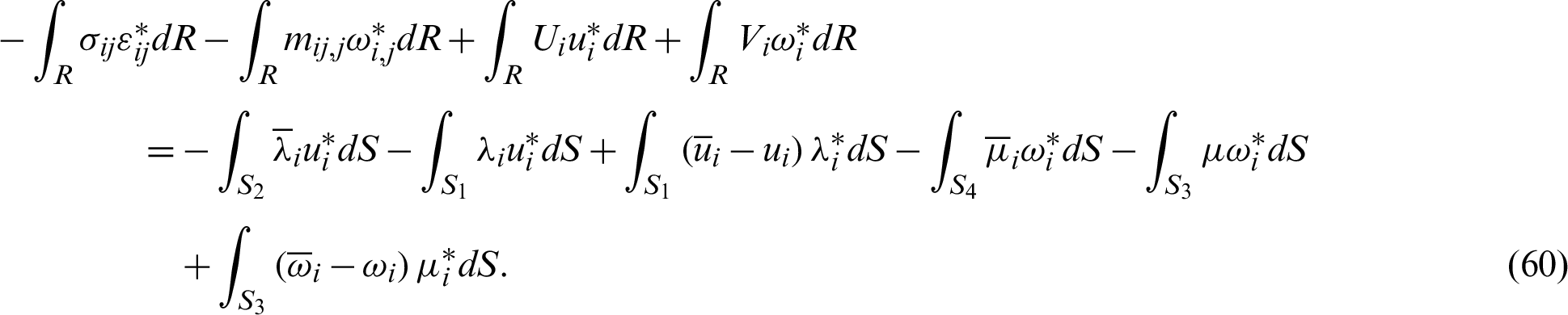
The memory dependent derivative governing equations for three-temperature nonlinear generalized anisotropic micropolar-thermoelasticity theory and its problems can be expressed as follows [27]


where


The two dimensions three temperature (2D-3T) radiative heat conduction equations can be expressed as


where  , mij,
  ,
,  , uk,
, uk,  and
and  are the mechanical stress tensor, couple stress, strain tensor, micro-strain tensor, displacement vector, temperature and reference temperature, respectively, Cabfg (Cabfg = Cfgab = Cbafg) and
  (
( ) are respectively, the constant elastic moduli and stress-temperature coefficients of the anisotropic medium, Fi, Mi and
  are mass force, mass couple and micro-rotation, respectively, J is micro-inertia coefficient,
 are the thermal conductivity coefficients, e, i and p denote electron, ion and phonon, respectively,
  is the second order tensor associated with the TEWED and TEWOED theories,
  ,
,  ,
,  ,
,  ,
,  and Å are the electron-ion energy coefficient, electron-phonon energy coefficient, density, specific heat capacities, time and unified parameter which introduced to consolidate all theories into a unified equations system, respectively,
 and
and  are the relaxation times, m is a functionally graded parameter. Also, g1, g2,
  and
and  are suitably prescribed functions,
  are the tractions defined by
 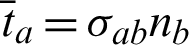 ,
,  and
and  are the Kronecker delta functions.
3 BEM Solution for Temperature Field
The 2D-3T radiative heat conduction equations mentioned above (15)–(17) coupled with electron, ion and phonon temperatures, can be expressed in the context of memory dependent derivative theory [27]


where


where
and

which can be written in memory dependent derivative form as follows
where

and

where  (i, j = 1, 2),
 and
and  are the Kronecker delta, delay times and kernel function, respectively.

Initial and boundary conditions of 3T field can be written as


By using the fundamental solutions  that satisfies the following differential equation

Now, by applying the technique of Fahmy [27] to (19) we can write

which, in the absence of heat sources, can be written as follows

In order to transform the domain integral of (33) into the boundary, the time derivative of temperature can be approximated as follows

where fj(r) are known functions and  are unknown coefficients.
We assume that  is a solution of

Then, Eq. (33) resulted in the following boundary integral equation

where

and

where  are the coefficients of
  that described as [50]

By discretizing Eq. (36) and using Eq. (38), we get [46]

where  is the heat flux vector and
  and
and  are matrices.
The diffusion matrix may be described as

where


To solve Eq. (41) numerically, the functions  and
and  have been interpolated as


where,  determines the practical time
  of the current time step.
By differentiating Eq. (44) with respect to time, we get

By substituting from Eqs. (44)–(46) into (40), we obtain

which can be written as follows

in which  represents unknown matrix while X and
  represent known matrices. The above formula gives the temperature as a function of the displacement field.
4 BEM Solution for Displacement Fields
Use of the weighted residual method to the governing Eqs. (9) and (10) yields


where


in which ui and  are approximate solutions and
  and
and  are weighting functions.
The boundary conditions are


By integrating the first term of Eqs. (49) and (50) by parts, we get


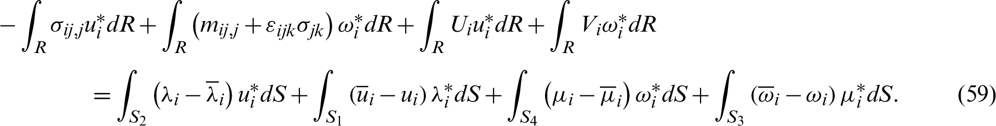
Based on Huang et al. [62], we can write the following boundary integral equation
By integrating the left-hand side of (59) by parts, we get
Based on Eringen [63], we can write

Thus, Eq. (60) can be reexpressed as
By integrating the left-hand side of (62) by parts again and neglecting body force Ui and body couple Vi, we get
The weighting functions for  and Vi = 0 along el direction can be obtained as:


Now, we consider the following analytic fundamental solution of Dragos [64]

The weighting functions for Ui = 0 and  along el direction can be expressed as:


The analytic fundamental solution of Dragos [64] can also be expressed as

By using the above weighting functions sets into (63) we have


Thus, we can write

where
In order to solve (72) numerically, we define the following functions

By substituting from (74) into (72), we get

which also can be written as

By applying the following definition

Thus, by using (77), we can write (76) as follows

Hence, the global matrix system can be expressed as

Now, by using the initial and boundary conditions, we can write (79) as follows

in which  represents unknown matrix while
  and
and  represent known matrices. An explicit staggered predictor-corrector algorithm which is based on the generalized modified shift-splitting (GMSS) iteration method [65] is implemented in order to solve (48) and (80) for obtaining the nonlinear three-temperature and nonlinear displacement fields.
5 Computational Performance of the Problem
Nowadays, modern CPUs are very powerful, versatile and can perform very complex problems much faster than previous ones [65,66]. We used GMSS method for the iterative solution of the resulted linear systems of equations  , where A is nonsingular, dense and nonsymmetric. We demonstrated the efficiency of our implemented GMSS method which results in fast convergence to the actual solution and does not need to complicated calculations.
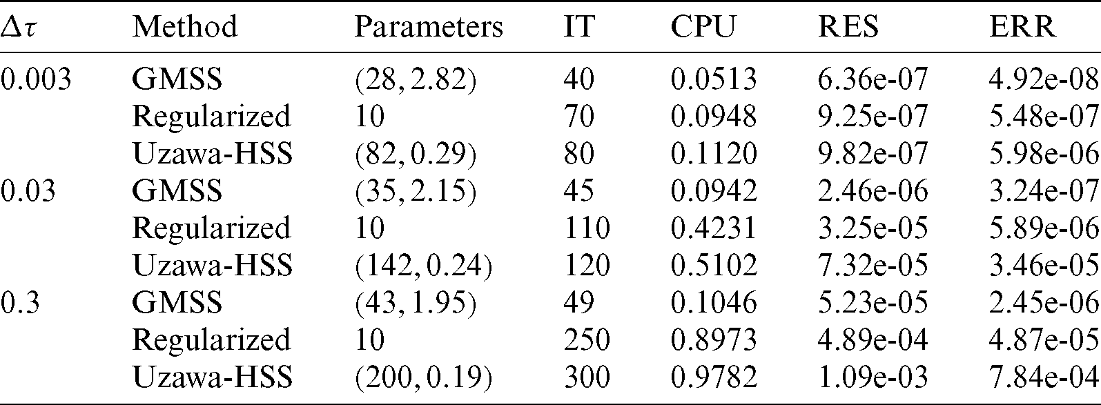
The main objective of this section is to implement an accurate and robust iteration technique for solving the dense nonsymmetric algebraic system of linear equations arising from the BEM. So, GMSS of Huang et al. [67] has been implemented for solving the resulting linear systems in order to reduce the number of iterations and the CPU time. The BEM discretization is employed 1280 quadrilateral elements, with 3964 degrees of freedom (DOF). The generalized modified shift-splitting (GMSS) iteration method of Huang et al. [67], Uzawa-HSS iteration method of Yang et al. [68] and regularized iteration method of Badahmane [69] were compared with each other in Tab. 1. From this table, one can see that GMSS efficiency is superior to other iteration methods.
Table 1: Numerical results for the tested iteration methods
5.1 Uzawa-HSS Iteration Method
Now, the resulted linear system  in Eqs. (48) and (80) can be considered in the following form

where  is a non-Hermitian positive definite coefficient matrix,
  is a full-column-rank matrix such that
  ,
,  is a known vector with
  and
and  .
.
The iteration scheme of Uzawa method can be defined as

Due to the effectiveness of Uzawa method, several generalized techniques of Uzawa method, such as parameterized Uzawa methods, preconditioned Uzawa methods, inexact Uzawa methods and parameterized inexact Uzawa methods, have been developed to solve (81).
In order to solve the linear system  , where, A is Hermitian positive definite matrix. Yun [70] developed three Uzawa methods based on one-step successive over relaxation (SOR) iteration method due to its high efficiency to approximate
  in each step of Uzawa method. Yang et al. [68] proposed the Uzawa-HSS iteration method based on one-step HSS iteration instead of one-step SOR. Bai et al. [71] proposed the Hermitian and skew-Hermitian splitting (HSS) iteration method to solve the non-Hermitian linear systems taking into consideration that
  where
where  and
and  are the Hermitian and skew-Hermitian matrices of A which can be written as

In order to describe the Uzawa-HSS, we consider the iteration scheme of HSS iteration method which is used for solving linear equations system  as follows

which equals to

where


Now, we can define the Uzawa–HSS iteration scheme as follows:
First, compute  from the following iteration scheme

Second, compute  from the following iteration scheme

where  is a Hermitian positive definite preconditioning matrix.
For  and
and  ,
,  until
until  and
and  converges, compute

where


5.2 Generalized Modified Shift-Splitting (GMSS) Iteration Method
Now, the resulted linear system (48) or (80) can be considered in the following form

where  and
and  ,
,  .
.
According to Cao et al. [72] and Zhou et al. [73] and based on the well-known Hermitian and skew-Hermitian splitting (HSS) of the matrix A  , of Bai et al. [71], the matrix
  can be written as

Now, the iteration scheme of the modified shift-splitting (MSS) can be described for solving linear equations system  , as
, as

Based on the MSS iteration method, the generalized modified shift-splitting (GMSS) for the nonsymmetric matrix  is derived as follows

For  ,
,  and
and  until
until  converges, compute

where  0,
0,  0 is, another given positive constant, and I is a unit matrix.
The GMSS iteration method can be expressed as

where

and

According to Huang et al. [67], who proposed the GMSS, we can write

Let  and
and  , where,
  ,
,  and
and  ,
, 
Now, the GMSS iteration method can be derived using the following algorithm:
For a given vector  , the vector
  can be computed from the following steps
Step 1. Compute 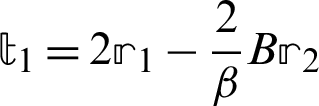 ,
,
Step 2. Solve 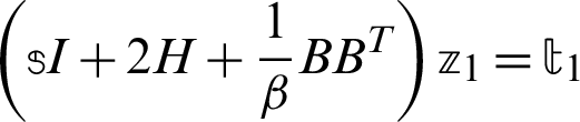 ,
,
Step 3. Compute 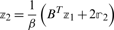 .
.
It can be seen from algorithm 1 that a linear system with the coefficient matrix 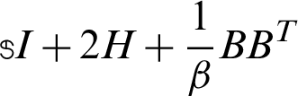 should be solved at each iteration, where the incomplete Cholesky factorization has been used as a preconditioner for Preconditioned Conjugate Gradient (PCG) Method for solving the sub-linear systems with the coefficient matrix
  .
.
5.3 Regularized Iteration Method
Badahmane [69] proposed a regularized iteration method for solving the following system

where  and
and  ,
,  .
.
According to Badahmane [69], the non-symmetric matrix  can be written as follows

For  ,
,  until
until  converges, compute

The GMSS iteration method can be expressed as

where

where the regularized preconditioner of the matrix  is
is

From (104), the regularized iteration method computes the approximate solutions of (102) by

which equals to

where  ,
,  and
and 
At each iteration step of regularized iteration (108), (109) should be solved using the following algorithm
1. Solve  where
where 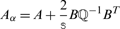 and
and 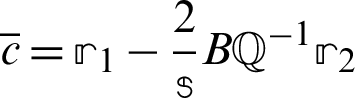
2. Compute 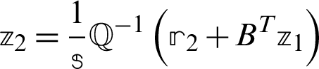 where
where  is a diagonal matrix,
 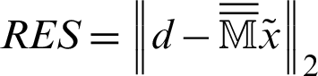 ,
,  ,
,  and
and  is the exact solution.
6 Numerical Results and Discussion
The technique proposed in the current study may be applicable to a wide variety of three-temperature micropolar-thermoelastic problems relating to the suggested theory. During the simulation process the effects of time-delay and kernel function play a very important role. The proposed technique has been proven to be successful and efficient.
In the considered boundary element model, the boundary has been discretized using 42 linear boundary elements and 68 internal points as shown in Fig. 2. Also, the FDM and FEM discretization of the domain has been performed using 1896 second order quadrilateral elements and 5986 nodes.
Figure 2: Boundary element model of the considered problem
Fig. 3 shows the variations of the nonlinear three-temperature ( ) along
  -axis for different values of time-delay
  and kernel function
  . It can be seen from this figure that the time-delay has a significant effect on the nonlinear three-temperature distribution.
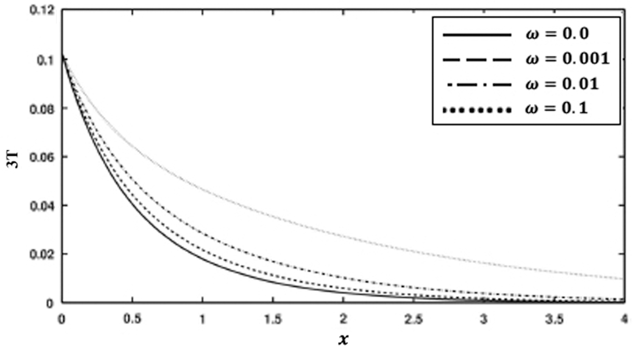
Figure 3: Variation of the  (
( ) along
  -axis for different values of time-delay
  and kernel function
  .
.
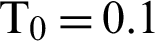
Figs. 4 and 5 show the variation of the nonlinear displacements u1 and u2 along  -axis for different values of time-delay
  and kernel function
  . It is clear from these figures that the time delay greatly affects the displacement components.
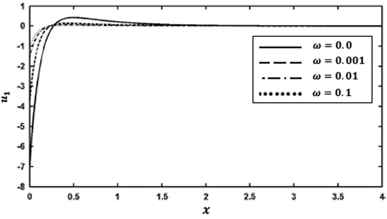
Figure 4: Variation of the displacement  along
along  -axis for different values of time-delay
  and kernel function
Figure 5: Variation of the displacement  along x-axis for different values of time-delay
  and kernel function
Fig. 6 shows the variation of the nonlinear three-temperature along  -axis for different forms of kernel function and time-delay
  . It is shown from this figure that the kernel function form has a significant influence on the nonlinear three-temperature distribution.
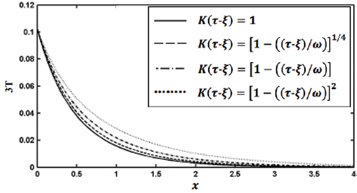
Figure 6: Variation of the temperature 3T (T0 = 0.1) along x-axis for different forms of kernel function and time-delay 
Figs. 7 and 8 show the variation of the nonlinear displacements u1 and u2 along  -axis for different forms of kernel function and time-delay
 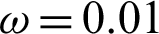 . It can be seen from these figures that the kernel function form has a significant influence on the nonlinear displacement components.
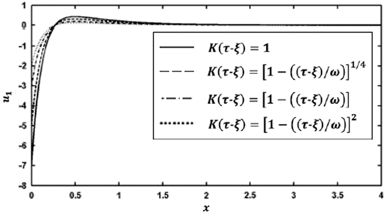
Figure 7: Variation of the displacement u1 along x-axis for different forms of kernel function and time-delay 
Figure 8: Variation of the displacement u2 along x-axis for different forms of kernel function and time-delay 
As there are no findings available for the problem under consideration. So, some literatures may be regarded as special cases from our general BEM problem. For comparison purposes with other approaches special cases addressed by other authors, we considered only one-dimensional problem. In the special case under consideration, the results are plotted in Figs. 9–11 to illustrate the total three-temperature and displacements distributions with the time  . The validity and exactness of our suggested technique have been demonstrated by a graphical comparison of the BEM special case results for the considered problem with those obtained using the FDM results of Pazera et al. [74] and FEM results of Xiong et al. [75] based on the substitution of three-temperature heat conduction with one-temperature heat conduction, it should be noted that the BEM results have been found to be in excellent agreement with the FDM and FEM results.
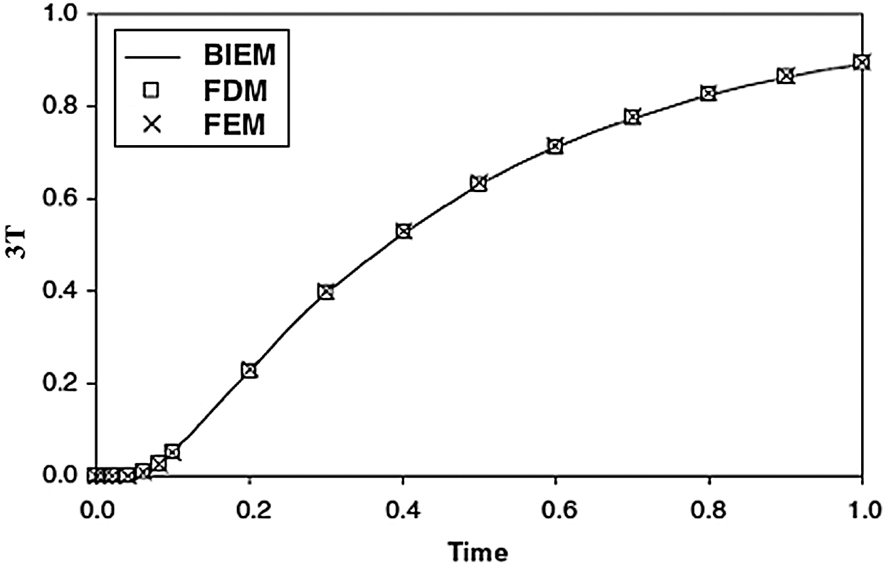
Figure 9: Variation of the nonlinear total temperature with time 
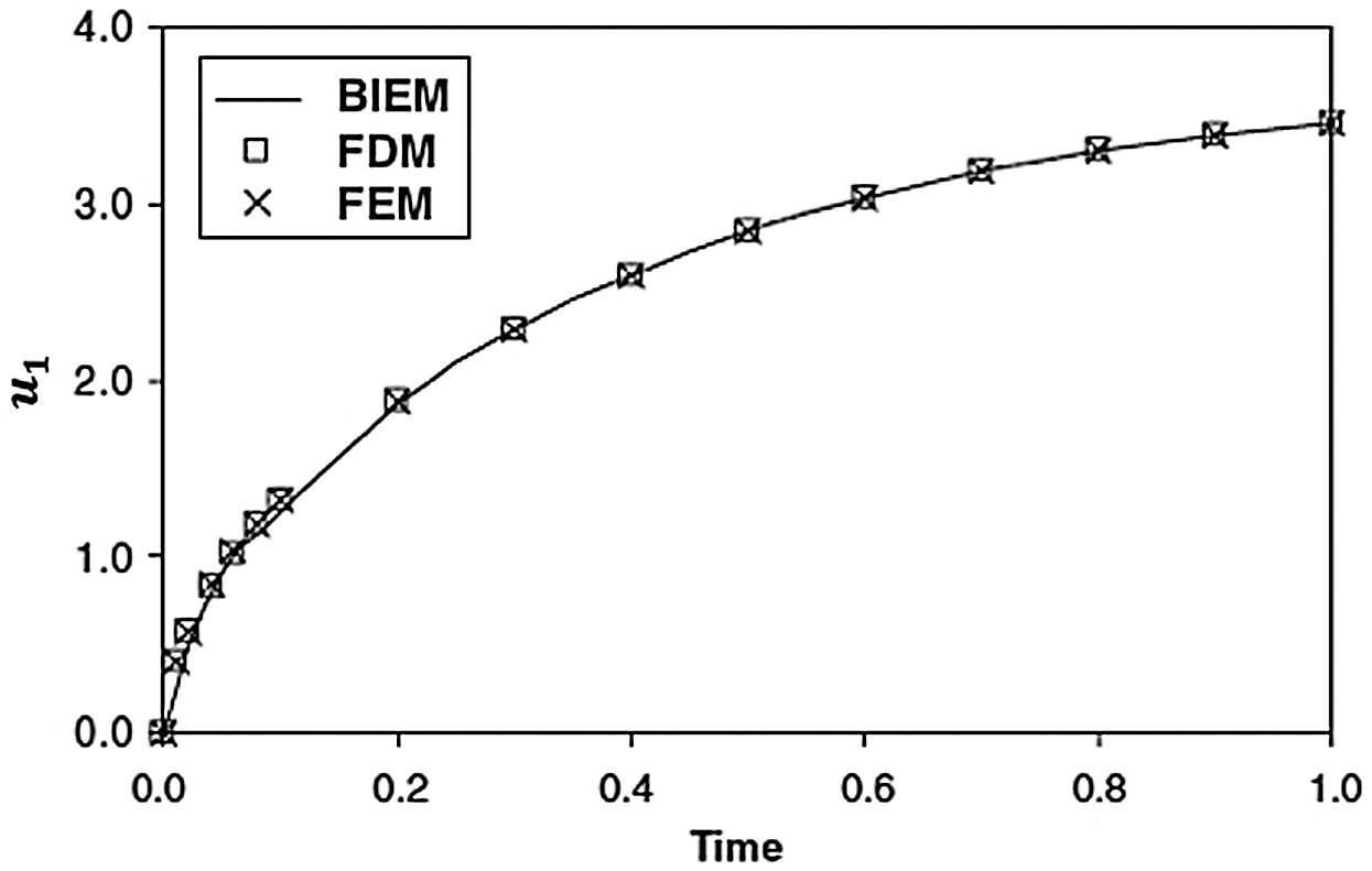
Figure 10: Variation of the nonlinear displacement  with time
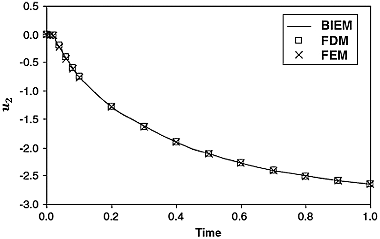
Figure 11: Variation of the nonlinear displacement  with time
The performance of GMSS iteration method is compared against Uzawa-HSS iteration method and regularized iteration method. In actual computation, the parameters,  for Uzawa-HSS iteration method,
  for GMSS iteration method and
  for regularized iteration method have been chosen to be the experimentally found optimal ones that minimize the total number of iterative steps of these methods. Tab. 1 reports the iteration number (IT), CPU time, relative residual (RES) and error (ERR) of the tested iteration methods with respect to different values of time-step size
  . From Tab. 1, it can be observed that the GMSS requires lowest IT and CPU times, which implies that the GMSS is superior to the other methods in terms of computing efficiency.
The main purpose of the current paper is to propose a new MDD theory called three-temperature nonlinear generalized anisotropic micropolar-thermoelasticity. This theory forms a new and good research point in thermoelasticity, and the scientific community will be interested in studying this research point in the following years due to its numerous low-temperature and high-temperature applications. The problems related to the proposed theory are very difficult to solve analytically. Therefore, we propose a new boundary element technique for solving such problems. For comparison purposes with other researchers in the literature, we only considered the one-dimensional one-temperature heat conduction model as a special case of our three-temperature heat conduction model. The numerical results confirm the validity and exactness of our suggested technique, where the BEM results are in excellent agreement with the results of FDM and FEM.
The GMSS iteration method has been implemented for solving the resulting linear systems in order to reduce the iterations number and CPU time. The implemented GMSS iteration method is quickly convergent without needing complicated calculations and. On the other hand, it is anticipated that the GMSS iteration method with the optimal parameters  would be much better and superior than Uzawa-HSS and regularized iteration methods for solving the resulting linear system from BEM. How to select the optimal parameters
  for GMSS iteration method is a very practical and interesting problem that still needs further research and can be suggested as a future work through the current study.
The numerical results of our considered study can provide data references for mechanical engineers, computer engineers, geotechnical engineers, geothermal engineers, technologists, new materials designers, physicists, material science researchers and those who are interested in novel technologies in the area of three-temperature micropolar generalized thermoelastic materials. Application of three-temperature theories in advanced manufacturing technologies, with the development of soft machines and robotics in biomedical engineering and advanced manufacturing, thermoelastic response will be encountered more often where three-temperature radiative heat conduction will turn out to be the best choice for thermomechanical analysis in the design and analysis of micropolar generalized thermoelastic materials and structures.
Acknowledgement: The authors would like to thank the anonymous reviewers and the editor for their useful suggestions and comments which gave rise to the opportunity to revise and improve this paper.
Funding Statement: The author received no specific funding for this study.
Conflict of Interest: The author declares that they have no conflicts of interest to report regarding the present study.
1. Lotfy, Kh. (2019). A novel model for photothermal excitation of variable thermal conductivity semiconductor elastic medium subjected to mechanical ramp type with two-temperature theory and magnetic field. Scientific Reports, 9, 3319. DOI 10.1038/s41598-019-39955-z. [Google Scholar] [CrossRef]
2. Lotfy, Kh. (2020). Analytical solutions of photo-thermal-elastic waves in a semiconductor material due to pulse heat flux with thermal memory. Silicon, 12(2), 263–273. DOI 10.1007/s12633-019-00120-w.
3. Abouelregal, A. E. (2019). Two-temperature thermoelastic model without energy dissipation including higher order time-derivatives and two phase-lags. Materials Research Express, 6(11), 116535. DOI 10.1088/2053-1591/ab447f.
4. Abouelregal, A. E. (2020). Generalized mathematical novel model of thermoelastic diffusion with four phase lags and higher-order time derivative. European Physical Journal Plus, 135(2), 263. DOI 10.1140/epjp/s13360-020-00282-2.
5. Abd-Alla A. M., Fahmy M. A., El-Shahat T. M. (2008). Magneto-thermo-elastic problem of a rotating nonhomogeneous anisotropic solid cylinder. Archive of Applied Mechanics, 78(2), 135–148. DOI 10.1007/s00419-007-0147-8.
6. Fahmy, M. A. (2008). Thermoelastic stresses in a rotating non-homogeneous anisotropic body. Numerical Heat Transfer, Part A: Applications, 53(9), 1001–1011. DOI 10.1080/10407780701789179.
7. Fahmy, M. A., El-Shahat, T. M. (2008). The effect of initial stress and inhomogeneity on the thermoelastic stresses in a rotating anisotropic solid. Archive of Applied Mechanics, 78(6), 431–442. DOI 10.1007/s00419-007-0150-0.
8. Fahmy, M. A. (2011). A time-stepping DRBEM for magneto-thermo-viscoelastic interactions in a rotating nonhomogeneous anisotropic solid. International Journal of Applied Mechanics, 3(4), 1–24. DOI 10.1142/S1758825111001202.
9. Fahmy, M. A. (2020). A new boundary element formulation for modeling and optimization of three-temperature nonlinear generalized magneto-thermoelastic problems of FGA composite microstructures. In: Chowdhury, M. A., Armenta, J. L. R., Rahman, M. M., Asiri, A. M., Inamuddin, (Eds.Composite Materials. London, UK: IntechOpen. [Google Scholar]
10. Duhamel, J. (1837). Some memoire sur les phenomenes thermo-mechanique. Journal de l’Ecole polytech, 15, 1–57. [Google Scholar]
11. Neumann, F. (1885). Vorlesungen Uber die theorie der elasticitat. Brestau: Meyer. [Google Scholar]
12. Biot, M. (1956). Thermoelasticity and irreversible thermo-dynamics. Journal of Applied Physics, 27(3), 249–253. [Google Scholar]
13. Lord, H. W., Shulman, Y. (1967). A generalized dynamical theory of thermoelasticity. Journal of the Mechanics and Physics of Solids, 15(5), 299–309. DOI 10.1016/0022-5096(67)90024-5. [Google Scholar] [CrossRef]
14. Green, A. E., Lindsay, K. A. (1972). Thermoelasticity. Journal of Elasticity, 2(1), 1–7. DOI 10.1007/BF00045689. [Google Scholar] [CrossRef]
15. Green, A. E., Naghdi, P. M. (1992). On undamped heat waves in an elastic solid. Journal of Thermal Stresses, 15(2), 253–264. DOI 10.1080/01495739208946136.
16. Green, A. E., Naghdi, P. M. (1993). Thermoelasticity without energy dissipation. Journal of Elasticity, 31(3), 189–208. DOI 10.1007/BF00044969. [Google Scholar] [CrossRef]
17. Fahmy, M. A. (2012). Transient magneto-thermoviscoelastic plane waves in a non-homogeneous anisotropic thick strip subjected to a moving heat source. Applied Mathematical Modelling, 36(10), 4565–4578. DOI 10.1016/j.apm.2011.11.036. [Google Scholar] [CrossRef]
18. Fahmy, M. A. (2012). Transient magneto-thermo-viscoelastic stresses in a rotating nonhomogeneous anisotropic solid with and without a moving heat source. Journal of Engineering Physics and Thermophysics, 85(4), 950–958. DOI 10.1007/s10891-012-0735-5.
19. Fahmy, M. A. (2012). Numerical modeling of transient magneto-thermo-viscoelastic waves in a rotating nonhomogeneous anisotropic solid under initial stress. International Journal of Modeling, Simulation and Scientific Computing, 3(2), 1250002. DOI 10.1142/S179396231250002X.
20. Fahmy, M. A. (2012). Transient magneto-thermo-elastic stresses in an anisotropic viscoelastic solid with and without moving heat source. Numerical Heat Transfer, Part A: Applications, 61(8), 547–564. DOI 10.1080/10407782.2012.667322.
21. Fahmy, M. A. (2012). The effect of rotation and inhomogeneity on the transient magneto-thermoviscoelastic stresses in an anisotropic solid. ASME Journal of Applied Mechanics, 79(5), 1015. DOI 10.1115/1.4006258.
22. Fahmy, M. A. (2013). A three-dimensional generalized magneto-thermo-viscoelastic problem of a rotating functionally graded anisotropic solids with and without energy dissipation. Numerical Heat Transfer, Part A: Applications, 63(9), 713–733. DOI 10.1080/10407782.2013.751317. [Google Scholar] [CrossRef]
23. Awrejcewicz, J., Grzelczyk, D. (2019). Dynamical systems theory. London, UK: IntechOpen. [Google Scholar]
24. Ebrahimi, F. (2019). Mechanics of functionally graded materials and structures. London, UK: IntechOpen.
25. Sivasankaran, S., Nayak, PK., Günay, E. (2020). Solid state physics–-metastable, spintronics materials and mechanics of deformable bodies. London, UK: IntechOpen.
26. Sadollah, A., Sinha, T. S. (2020). Recent trends in computational intelligence. London, UK: IntechOpen. [Google Scholar]
27. Fahmy, M. A. (2019). A new boundary element strategy for modeling and simulation of three temperatures nonlinear generalized micropolar-magneto-thermoelastic wave propagation problems in FGA structures. Engineering Analysis with Boundary Elements, 108, 192–200. DOI 10.1016/j.enganabound.2019.08.006. [Google Scholar] [CrossRef]
28. Cattaneo, C. (1958). Sur une forme de i’equation de la chaleur elinant le paradox d’une propagation instantanc. Comptes rendus de l’Académie des Sciences, 247, 431–433. [Google Scholar]
29. Oldham, K. B., Spanier, J. (2006). The fractional calculus: theory and applications of differentiation and integration to arbitrary order. Mineola: Dover Publication. [Google Scholar]
30. Soukkou, A., Belhour, M. C., Leulmi, S. (2016). Review, design, optimization and stability analysis of fractional-order PID controller. International Journal of Intelligent Systems and Applications, 8(7), 73–96. DOI 10.5815/ijisa.2016.07.08. [Google Scholar] [CrossRef]
31. Kilbas, A. A., Srivastava, H. M., Trujillo, J. J. (2006). Theory and applications of fractional differential equations. Netherlands: Elsevier Science.
32. Sabatier, J., Agrawal, O. P., Machado, J. A. T. (2007). Advances in fractional calculus: Theoretical developments and applications in physics and engineering. Netherlands: Springer. [Google Scholar]
33. Diethelm, K. (1997). Generalized compound quadrature formulae for finite-part integrals. IMA Journal of Numerical Analysis, 17(3), 479–493. DOI 10.1093/imanum/17.3.479. [Google Scholar] [CrossRef]
34. Wang, J. L., Li, H. F. (2011). Surpassing the fractional derivative: Concept of the memory-dependent derivative. Computers and Mathematics with Applications, 62(3), 1562–1567. DOI 10.1016/j.camwa.2011.04.028. [Google Scholar] [CrossRef]
35. Fahmy, M. A. (2013). Implicit-explicit time integration DRBEM for generalized magneto-thermoelasticity problems of rotating anisotropic viscoelastic functionally graded solids. Engineering Analysis with Boundary Elements, 37(1), 107–115. DOI 10.1016/j.enganabound.2012.08.002. [Google Scholar] [CrossRef]
36. Fahmy, M. A. (2013). Generalized magneto-thermo-viscoelastic problems of rotating functionally graded anisotropic plates by the dual reciprocity boundary element method. Journal of Thermal Stresses, 36(3), 1–20. DOI 10.1080/01495739.2013.765206. [Google Scholar] [CrossRef]
37. El-Naggar, A. M., Abd-Alla, A. M., Fahmy, M. A., Ahmed, S. M. (2002). Thermal stresses in a rotating non-homogeneous orthotropic hollow cylinder. Heat and Mass Transfer, 39(1), 41–46. DOI 10.1007/s00231-001-0285-4. [Google Scholar] [CrossRef]
38. El-Naggar, A. M., Abd-Alla, A. M., Fahmy, M. A. (2003). The propagation of thermal stresses in an infinite elastic slab. Applied Mathematics and Computation, 157(2), 307–312. DOI 10.1016/j.amc.2003.08.116.
39. Abd-Alla, A. M., El-Naggar, A. M., Fahmy, M. A. (2003). Magneto-thermoelastic problem in non-homogeneous isotropic cylinder. Heat and Mass Transfer, 39(7), 625–629. DOI 10.1007/s00231-002-0370-3. [Google Scholar] [CrossRef]
40. Zhang, Y., Yin, B., Cao, Y., Liu, Y., Li, H. (2020). A numerical algorithm based on quadratic finite element for two-dimensional nonlinear time fractional thermal diffusion model. Computer Modeling in Engineering & Sciences, 122(3), 1081–1098. DOI 10.32604/cmes.2020.07822. [Google Scholar] [CrossRef]
41. El Kahoui, A., Malek, M., Izem, N., Mohamed, M. S., Seaid, M. (2020). Partition of unity finite element analysis of nonlinear transient diffusion problems using p-version refinement. Computer Modeling in Engineering & Sciences, 124(1), 61–78. DOI 10.32604/cmes.2020.010874.
42. Sur, A., Pal, P., Mondal, S., Kanoria, M. (2019). Finite element analysis in a fiber-reinforced cylinder due to memory-dependent heat transfer. Acta Mechanica, 230(5), 1607–1624. DOI 10.1007/s00707-018-2357-2. [Google Scholar] [CrossRef]
43. Wang, Q., Zhou, W., Cheng, Y., Ma, G., Chang, X. (2017). A line integration method for the treatment of 3D domain integrals and accelerated by the fast multipole method in the BEM. Computational Mechanics, 59(4), 611–624. DOI 10.1007/s00466-016-1363-2. [Google Scholar] [CrossRef]
44. Brebbia, C. A., Dominguez, J. (1977). Boundary element methods for potential problems. Applied Mathematical Modelling, 1(7), 372–378. DOI 10.1016/0307-904X(77)90046-4.
45. Liang, K. Z., Huang, F. Y. (1996). Boundary element method for micropolar elasticity. International Journal of Engineering Science, 34(5), 509–521. DOI 10.1016/0020-7225(95)00110-7.
46. Brebbia, C. A., Telles, J. C. F., Wrobel, L. (1984). Boundary element techniques in engineering. New York: Springer-Verlag. [Google Scholar]
47. Wrobel, L. C., Brebbia, C. A. (1987). The dual reciprocity boundary element formulation for nonlinear diffusion problems. Computer Methods in Applied Mechanics and Engineering, 65(2), 147–164. DOI 10.1016/0045-7825(87)90010-7.
48. Kakuba, G., Mango, J. M. (2019). Anthonissen MJH. Convergence properties of local defect correction algorithm for the boundary element method. Computer Modeling in Engineering & Sciences, 119(1), 207–225. DOI 10.32604/cmes.2019.04269.
49. Fahmy, M. A. (2020). Boundary element algorithm for nonlinear modeling and simulation of three-temperature anisotropic generalized micropolar piezothermoelasticity with memory-dependent derivative. International Journal of Applied Mechanics, 12(3), 2050027. DOI 10.1142/S1758825120500271.
50. Fahmy, M. A. (2020). A new convolution variational boundary element technique for design sensitivity analysis and topology optimization of anisotropic thermo-poroelastic structures. Arab Journal of Basic and Applied Sciences, 27(1), 1–12. DOI 10.1080/25765299.2019.1703493. [Google Scholar] [CrossRef]
51. Fahmy, M. A. (2018). Shape design sensitivity and optimization for two-temperature generalized magneto-thermoelastic problems using time-domain DRBEM. Journal of Thermal Stresses, 41(1), 119–138. DOI 10.1080/01495739.2017.1387880.
52. Fahmy, M. A. (2019). Boundary element modeling and simulation of biothermomechanical behavior in anisotropic laser-induced tissue hyperthermia. Engineering Analysis with Boundary Elements, 101, 156–164. DOI 10.1016/j.enganabound.2019.01.006.
53. Fahmy, M. A. (2019). A new LRBFCM-GBEM modeling algorithm for general solution of time fractional order dual phase lag bioheat transfer problems in functionally graded tissues. Numerical Heat Transfer, Part A: Applications, 75(9), 616–626. DOI 10.1080/10407782.2019.1608770.
54. Fahmy, M. A. (2019). Design optimization for a simulation of rotating anisotropic viscoelastic porous structures using time-domain OQBEM. Mathematics and Computers in Simulation, 66, 193–205. DOI 10.1016/j.matcom.2019.05.004.
55. Fahmy, M. A. (2018). Boundary element algorithm for modeling and simulation of dual-phase lag bioheat transfer and biomechanics of anisotropic soft tissues. International Journal of Applied Mechanics, 10(10), 1850108. DOI 10.1142/S1758825118501089.
56. Fahmy, M. A. (2012). A time-stepping DRBEM for the transient magneto-thermo-visco-elastic stresses in a rotating non-homogeneous anisotropic solid. Engineering Analysis with Boundary Elements, 36(3), 335–345. DOI 10.1016/j.enganabound.2011.09.004.
57. Fahmy, M. A. (2014). A computerized DRBEM model for generalized magneto-thermo-visco-elastic stress waves in functionally graded anisotropic thin film/substrate structures. Latin American Journal of Solids and Structures, 11(3), 386–409. DOI 10.1590/S1679-78252014000300003. [Google Scholar] [CrossRef]
58. Cheng, A. H. D., Cheng, D. T. (2005). Heritage and early history of the boundary element method. Engineering Analysis with Boundary Elements, 29(3), 268–302. DOI 10.1016/j.enganabound.2004.12.001. [Google Scholar] [CrossRef]
59. Sladek, V., Sladek, J. (1985). Boundary element method in micropolar thermoelasticity. Part I: Boundary integral equations. Engineering Analysis, 2(1), 40–50. DOI 10.1016/0264-682X(85)90050-4. [Google Scholar] [CrossRef]
60. Sladek, V., Sladek, J. (1985). Boundary element method in micropolar thermoelasticity. Part II: Boundary integro-differential equations. Engineering Analysis, 2(2), 81–91. DOI 10.1016/0264-682X(85)90058-9.
61. Sladek, V., Sladek, J. (1985). Boundary element method in micropolar thermoelasticity. Part III: Numerical solution. Engineering Analysis, 2(1), 155–162. DOI 10.1016/0264-682X(85)90021-8. [Google Scholar] [CrossRef]
62. Huang, F. Y., Liang, K. Z. (1996). Boundary element method for micropolar thermoelasticity. Engineering Analysis with Boundary Elements, 17(1), 19–26. DOI 10.1016/0955-7997(95)00086-0. [Google Scholar] [CrossRef]
63. Eringen, A. C. (1968). Theory of micropolar elasticity. In: Liebowitz, H., (Ed.Fracture. New York: Academic Press. [Google Scholar]
64. Dragos, L. (1984). Fundamental solutions in micropolar elasticity. International Journal of Engineering Science, 22(3), 265–275. DOI 10.1016/0020-7225(84)90007-7. [Google Scholar] [CrossRef]
65. Chronopoulos, A. T., Gear, C. W. (1989). S-step iterative methods for symmetric linear systems. Journal of Computational and Applied Mathematics, 25(2), 153–168. DOI 10.1016/0377-0427(89)90045-9. [Google Scholar] [CrossRef]
66. Ma, S., Chronopoulos, A. T. (1990). Implementation of iterative methods for large sparse non-symmetric linear systems on a parallel vector machine. International Journal of High Performance Computing Applications, 4(4), 9–24. [Google Scholar]
67. Huang, Z. G., Wang, L. G., Xu, Z., Cui, J. J. (2017). The generalized modified shift-splitting preconditioners for nonsymmetric saddle point problems. Applied Mathematics and Computation, 299, 95–118. DOI 10.1016/j.amc.2016.11.038. [Google Scholar] [CrossRef]
68. Yang, A. L., Wu, Y. J. (2014). The Uzawa–HSS method for saddle-point problems. Applied Mathematics Letters, 38, 38–42. DOI 10.1016/j.aml.2014.06.018. [Google Scholar] [CrossRef]
69. Badahmane, A. (2020). Regularized preconditioned GMRES and the regularized iteration method. Applied Numerical Mathematics, 152, 159–168. DOI 10.1016/j.apnum.2020.01.001. [Google Scholar] [CrossRef]
70. Yun, J. H. (2013). Variants of the Uzawa method for saddle point problem. Computers & Mathematics with Applications, 65(7), 1037–1046. DOI 10.1016/j.camwa.2013.01.037. [Google Scholar] [CrossRef]
71. Bai, Z. Z., Golub, G. H., Ng, M. K. (2002). Hermitian and skew-hermitian splitting methods for non-hermitian positive definite linear systems. SIAM Journal on Matrix Analysis and Applications, 24(3), 603–626. DOI 10.1137/S0895479801395458. [Google Scholar] [CrossRef]
72. Cao, Y., Du, J., Niu, Q. (2014). Shift-splitting preconditioners for saddle point problems. Journal of Computational and Applied Mathematics, 272, 239–250. DOI 10.1016/j.cam.2014.05.017. [Google Scholar] [CrossRef]
73. Zhou, S. W., Yan, A. L., Dou, Y., Wu, Y. J. (2016). The modified shift-splitting preconditioners for nonsymmetric saddle-point problems. Applied Mathematics Letters, 59, 109–114. DOI 10.1016/j.aml.2016.03.011. [Google Scholar] [CrossRef]
74. Pazera, E., Jedrysiak, J. (2018). Effect of microstructure in thermoelasticity problems of functionally graded laminates. Composite Structures, 202, 296–303. DOI 10.1016/j.compstruct.2018.01.082. [Google Scholar] [CrossRef]
75. Xiong, Q. L., Tian, X. G. (2015). Generalized magneto-thermo-microstretch response during thermal shock. Latin American Journal of Solids and Structures, 12(13), 2562–2580. DOI 10.1590/1679-78251895. [Google Scholar] [CrossRef]
 | This work is licensed under a Creative Commons Attribution 4.0 International License, which permits unrestricted use, distribution, and reproduction in any medium, provided the original work is properly cited. |