Computer Modeling in Engineering & Sciences

DOI: 10.32604/cmes.2021.011163

ARTICLE

Multiquadric Radial Basis Function Approximation Scheme for Solution of Total Variation Based Multiplicative Noise Removal Model

Mushtaq Ahmad Khan1,*, Ahmed B. Altamimi2, Zawar Hussain Khan3, Khurram Shehzad Khattak3, Sahib Khan4,*, Asmat Ullah3 and Murtaza Ali1

1University of Engineering and Technology, Mardan, 23200, Pakistan
2University of Hail, Hail, Saudi Arabia
3University of Engineering and Technology, Peshawar, 25000, Pakistan
4Politecnico di Torino, Torino, 10129, Italy
*Corresponding Authors: Mushtaq Ahmad Khan. Email: mushtaq@uetmardan.edu.pk; Sahib Khan. Email: sahib.khan@polito.it
Received: 23 April 2020; Accepted: 19 August 2020

1  Introduction

Image denoising performs a significant part in the fields of image processing and mathematics. We referred the readers [1,2] for further information. Image noise is classified into two major types, i.e., additive and multiplicative noises. This type of noise which is independent of the signal intensity and independent at each pixel is called Additive Gaussian noise. It is caused primarily by thermal noise in the electronic components of digital cameras. A special case in which the values at any pair of times are identically distributed and statistically independent is called White Gaussian noise. Although Gaussian noise and speckle noise can look externally comparable in an image, they are a consequence of various methods and need several strategies for their dismissal. Although Gaussian noise can be formulated by random values combined with the pixel values of an image, speckle noise is modeled by arbitrarily selected values that are multiplied by the pixel values. Speckle noise is an important difficulty that appeared in some radar applications. Another basic sort of noise is data drop-out noise, usually related to as impulse noise or salt-and-pepper noise. Hereabouts, the noise is generated by errors in data transmission. Degraded pixels are either set to the maximum value or to zero, producing the image a salt and pepper-like appearance. Unconcerned pixels remain constant. The noise is usually quantified by the percentage of pixels that are contaminated [3].

Most of the image denoising literature is connected with the additive noise model:

where f is given the noisy image degraded by additive noise , and u is the restored image. A variety of strategies have been utilized to handle the aforementioned issue like wavelet approaches [4,5], stochastic approaches [6], and variational approaches [7–11]. In this study, we are mainly concentrated on the image denoising problems connected with multiplicative noise, which is modeled as below:

where f: , represents the degraded image containing multiplicative noise and u represents the true image. The notation describes the image domain which is usually a rectangular domain. Multiplicative noise is one of the most complicated image noise models. It is signal independent, non-Gaussian, and spatially dependent. Consequently, multiplicative denoising is a highly challenging task compared with the additive Gaussian noise. Numerous image denoising tasks connected with multiplicative noise have been suggested by the researchers in various disciplines, particularly in Synthetic Aperture Radar (SAR) and Medical Sciences, for more information, see [12–17]. In image denoising literature, several mesh-based schemes such as Split Bregman scheme [7], Linearized gradient scheme [18], Operator Splitting scheme [8], Multigrid scheme [19], Level set approach [20], etc. have been used by the researchers to solve the models and to remove the multiplicative noise from the images. For more information, see [10,11,21–28].

In recent years, TV-based filtering [18,22] has been found as a famous regularization filter for image restoration for variational PDE-based models. In the image regularization process, it is assumed that the image is taken on a continuous region, which appears in continuous functional and then results in the Euler–Lagrange restoration equation. The traditional mash-based schemes are applied on Euler–Langrage PDE to discretize on a regular gird for the most suitable solution. For more details, see [29–31]. The main disadvantage associated with the solution of TV-based models by traditional mesh-based numerical techniques results in the transformation of smooth functions toward piece-wise constant functions. This appearance of transformation is remembered as the staircase effect, which generates images to appear blocky. Another disadvantage of these mesh-based methods is that the surface of the picture (texture) is also effected by noise during the denoising process. Furthermore, the classical mesh-based methods are normally time-consuming and struggle with smooth solutions of the Euler Lagrange PDEs associated the minimization functional of TV-based models due to the non-linearity and non-differentiability.

In the last many decades, meshless schemes have been witnessed as an interesting field of research by the researchers for solving PDEs. Meshless scheme based on RBFs is a completely meshless approach for solving PDEs. In a meshless (meshfree) approach a set of scattered nodes [32] is employed rather than meshing the domain of the problem. The performance of RBFs as a meshless technique for the numerical solution of PDEs is depended upon the collocation method. Because of the collocation technique, this approach does not require to estimate any integral. The principal benefit of numerical methods, which apply radial basis functions over conventional techniques, is the meshless characteristic of these methods which occurs in superior performance in spectral accuracy [33] and exponential convergence [34] of RBFs collocation methods corresponded to the classical mesh-based numerical approaches such as Finite Difference Scheme (FDM) [35], Finite Element Scheme (FEM) [36], Finite Volume Scheme (FVM) [19,37], and Pseudo-Spectral Scheme [38]. For more details regarding RBF interpolation schemes, see [39–43].

RBF scheme has been studied as a global collocation technique that is simple to implement, converges exponentially, and contributes good accuracy [44] in solving PDEs. The meshless scheme is (conditionally) Positive Definite (PD) [34,45] and rotationally invariant which is responsible for unique solutions through the interpolation process. Recently, the RBF collocation scheme has been utilized on noticed random data points to remove the Gibbs oscillation [46]. Although the interpolation matrix achieved during the RBF collocation method is completely populated, ill-conditioned, and hence computationally expensive when applied to large scale data. The interpolation matrix is also based on the value of the shape parameter connected with the basis function. Kansa introduced the RBF collocation meshless scheme while Hardy used Multiquadric (MQ) as a basis function in the Kansa scheme (Collocation scheme) to solve PDEs [47,48]. In brief, the Kansa collocation scheme had been practiced for the smooth numerical solution of hyperbolic and elliptic equations such as the linear advection-diffusion equation and the Poisson equation and consequently some beneficial numerical results have been achieved compared to finite difference method [49,50].

Motivated by the RBF collocation method (Kansa method) applied to the numerical solution of PDEs, this research work proposes to implement the Kansa technique (RBF collocation method) on nonlinear Euler–Lagrange restoration equation connected with the minimization functional of TV-based model and to get the smooth solution regarding image restoration. The recommended meshless algorithm will be capable of removing the noise, elimination of the staircase effects, preservation of edges, textures, and fine details from images during the reconstruction process. The principal utilization of the recommended meshless algorithm in image denoising is; the Multiquadric radial basis function (MQ-RBF) interpolation process utilized in the suggested meshless algorithm will not only effective in edge preservation but will also essential in fine details, while the smooth solution and the lack of dependency on a mesh or integration application will result in excellent denoising results in terms of texture preservation and reduction of staircase effect.

The outlines of this article are as follows. Section 2, introduces the TV-regularization utilized in image denoising. This section also includes a detailed review of RBF approximation used in PDEs solution. Section 3, describes Huang et al. [22] model adopted for the removal of multiplicative noise. Section 4, demonstrates the detailed Mathematical discussion of the mesh-based scheme used for the numerical solution of Huang et al. model. This section also describes the complete mathematical formulation of the proposed meshless collocation scheme (Kansa scheme) employed for the numerical solution of PDE associated with the minimization functional of Huang et al. model. The numerical results are summarized in Section 5 to validate the effectiveness of the proposed meshless algorithm concerning the image restoration quality (Peak Signal to Noise Ratio (PSNR), Signal to Noise Ratio (SNR), and Mean Structure Similarity (MSSIM) index), iterative numbers, and computational speed compared to some traditional TV-based mesh-based algorithms. The tabulated analysis of parameter sensitivity examination is provided in Section 6. A brief conclusion is presented in Section 7. Finally, the detailed derivatives of the proposed algorithm are presented in an appendix.

2  Mathematical Background

2.1 Total Variation Filtering in Image Denoising

The TV regularization is a technique in digital image processing used for the solution of inverse problems and numerical [51]. This technique has the advantage of removing the noise from the given noisy image data while preserving important details such as edges. Let be selected in 2D space over domain . Then the Total variation (TV) variation regarding the image is written as:

The TV-based minimization functional presented by Huang et al. [18] to remove the multiplicative noise (2) is addressed by the following formula.

In the above Eq. (4), the primary part is known as the regularization part of u, while the second part is known as fitting/fidelity part and and are two fitting parameters. Numerous TV-based conventional schemes have been introduced to resolve the minimization functional (4), for example, see [18,22,52].

2.2 Radial Basis Functions Approximation

Let us define the RBF approach [53,54]. The Radial basis function is a function concerning the origin or on the distance between a presented point and data set with , while is called as radial function. Some examples of commonly continuous differentiable RBFs are displayed in the Tab. 1. The RBF procedure is employed to interpolate a function f(x) smoothly for a closed domain with . For the given N data points and data center points, the RBF interpolation of f(x) is mentioned by the following form:

where are unknown weights and are achieved by solving the given over determined linear system of equations.

which leads to the following linear system of equations.

where represents the unknown vector and to be determined while , represents known vector, and

is known as interpolation matrix. To guarantee the invariability of the interpolation matrix A, the polynomial part is increased to the RBF Eq. (5). Consequently, Eq. (5) is re-defined as follow:

with constraints

where indicates the polynomial including m in N total degree variables polynomials [45] with , which is described as given.

Table 1: [k] indicates the most neighboring integers less than or equivalent to k, N denotes a natural number, while c indicates shape parameter associated with RBFs, and conditionally positive definite function of order m is expressed by CPD [53,57]

The consolidated solution of Eqs. (9) and (10) through interpolation process leads to the given matrix system of linear equations.

where shows the system matrix containing A, as elements of the system in the forms of P, and O is null matrics.

The shape parameter c connected with RBFs, the definiteness of RBFs i.e., positive definiteness (PD), and conditionality positive definiteness (CPD) are provided in Tab. 1 and reviewed in [45,55,56].

3  Li–Li Huang Model

The first Weberized TV regularization based variational model for removing the multiplicative noise from provided degraded image was presented by Huang et al. [18]. The minimization methodology of the model (2) by applying [18] is written mathematically by the subsequent equation.

where

is described as the regularization part. The primary part in the regularization part is recognized as TV term while the second part is recognized as Weberized TV term which is presented as under:

The minimization approach of Eq. (13) by [18] is defined as:

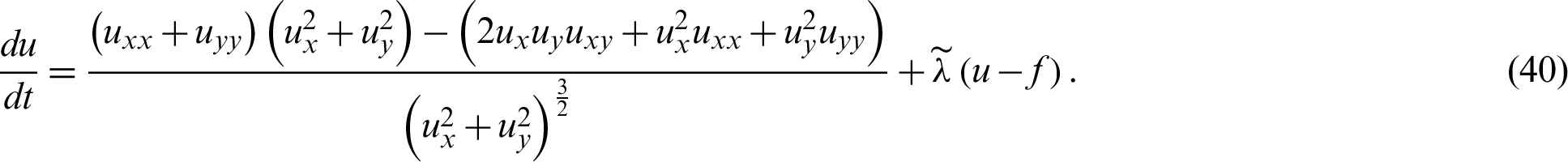
where the first term is known as the total variation of u and and are the two regularization parameters while the second term is called data fitting term, sequentially. All these regularization parameters and are applied to balance the restoration and smoothness of the restored image which normally based on the image size and noise level. Here f > 0 in is the given data in the model. Since u > 0, the solution of functional (16) then produces the resulting Euler–Lagrange equation.

Define , then Eq. (17) can be re-written as;

or

for the given u(x, y, 0), and also on . For further details, the readers are referred to [18].

4  Numerical Schemes

In this section, we show some numerical approaches for solving nonlinear PDE (18) or (19) connected with the minimization functional (16).

4.1 Mesh-Based Scheme (M1)

Huang et al. [18] introduced a conventional mesh-based scheme for the numerical solution of nonlinear PDE (18) which is written as follows.

The foregoing Eq. (18) can also be re-written below.

which is the same as the TV classical denoising equation [29,58], while depends on u. The operator form of Eq. (21) is given as follows:

where L(u) represents the linear diffusion operator whose operation on function u is given by following equation.

The fixed point iterative scheme is utilized on (22) and is written as:

The finite difference method is used to discretize the PDE (24) by similar lines as done in [18]. The numerical solution of Eq. (24) is given as follows.

where , h is recognized as space step size and its value is chosen as h = 1, and is called regularized parameter and its value is selected . The conjugate gradient method is applied to solve the Eq. (24). For more information, the readers are referred to [18].

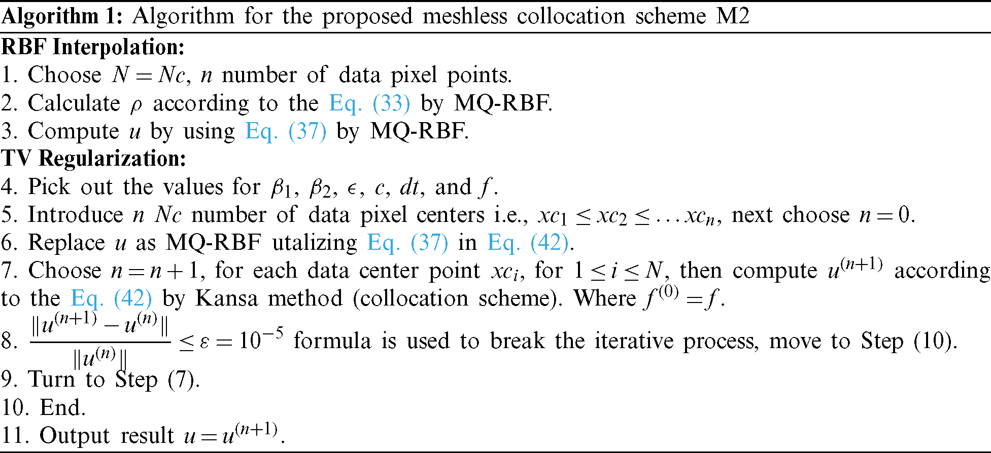
4.2 Proposed Meshless Scheme (M2)

In this subsection, the meshless collocation scheme is introduced for the numerical solution of Euler–Lagrange PDE (19) by employing RBF interpolation connected with the minimization of TV-based functional (16). The suggested meshless algorithm is not only expected to restore the images well and minimize the staircase effect but also the advantage to preserve the sharp edges and textures. Therefore, by using the proposed meshless scheme, consistent improvement in PSNR values, SNR values, and SSIM are expected to obtain. Assume be Nc data centers in a closed domain with RBF equation in R2, i.e., r = (x, y). Consequently, for the given known Nc data center points, the polynomial term free RBF interpolation is written as follows.

The coefficients of in the preceding Eq. (29) is achieved by utilizing the following interpolation condition.

with a bunch of points that agree to the centers Nc. The RBF interpolation at Nc data centers is presented through the given overdetermined interpolation form:

which produces linear system of equations and is applied to solve the coefficients , where and represent order matrices. In the above Eq. (31), C is recognized as square interpolation or system matrix and is represented by the following form:

In addition, matrix C in Eq. (31) is invertible [45,59] as it is positive definite [53,60] which is an critical aspect for unique solution of Eq. (31). Thus

Furthermore, at () N evaluation data points, the BRF interpolation by applying Eq. (29) give matrix D which is written as follows.

Also, N data points the interpolation over determined condition is estimated by applying the matrix-vector product to generate u and is described as below:

Combining Eqs. (33) and (35) result in the given equation.

or

which describes the estimated solution at any point in . Where u is of order matrix.

Since Eq. (19) is

The time marching restoration PDE [18] from (38) mentioned by the following equation:

for the given u(x, y, 0) with on . The Eq. (39) is re-written as

The semi implicit gradient decent scheme is then applied on the Eq. (40) and hence we get the following equation.

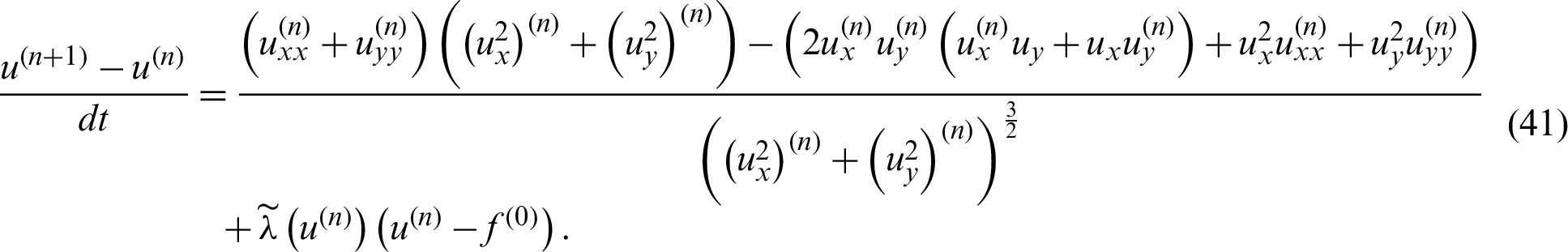
Combination the restoration Eq. (41) with Eq. (37) result in nonlinear restoration system of equations which is determined by the collocation approach (Kansa method). The Gauss–Jacobi iterative scheme is utilized in Kansa method to resolve the nonlinear restoration system of equations and is formulated by the given equation:

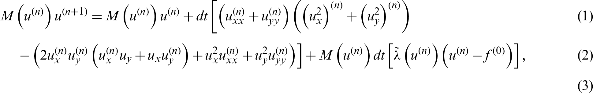
where , ux = Sxf, 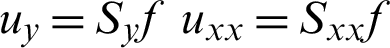, uyy = Syyf, , and f(0) = f.

Since the RBF in the RBF collocation technique (Kansa method) does not only fundamentally fulfill the resultant Euler Lagrange Eq. (42), but has more independence to choose an RBF. The most famous RBF in the Kansa technique is the multiquadric (MQ) [48,60], which normally displays spectral accuracy if an appropriate value of shape parameter c is chosen. In scheme M2, the shape parameter c and regularization parameters and depend upon the size and noise of the examined image. The main application of the collocation scheme employed on Eq. (42) results in a novel solution of (42) because of the MQ-RBF interpolation process used in Kansa technique M2 which leads to the preservation of the edges. Moreover, the weighted mean obtained from Eq. (31) through the interpolation approach is responsible for the smooth solution of the resultant Eq. (42) which depends upon the Euclidean distance between a noisy pixel and other non-noisy pixels acquired from Eq. (29) in the accepted framework. Consequently, the smooth solution obtained from Eq. (42) is tied to image reconstruction, eliminating the staircase effect, and maintaining edges, textures, and image details.

The proper determination of regularization parameters in the regularization process normally utilized to adjust the data fitting and regularization terms in the regularization models. Additionally, it may also not possible to pick a fixed parameter for various scale features like in-homogeneous distribution of cartoon, texture, and small details in an image. This recommends that spatially dependent weight functions/parameters, i.e., and c depend on u are reported to good quality outcomes. For this purpose, we select the value of and c manually by “Trial and Error Method and experienced the most substantial denoising results both visually and peak signal-to-noise ratio, signal-to-noise ratio, and structural similarity index efficiently. Hence, we choose and c as follows.

where , since u > 0, and , while c > 0. We conclude that there are two regularization parameters and and shape parameter c in the recommended meshless technique M2 which controls the trade-off between the regularization and image filtering term. Additionally, the acceptable values in the preceding rule are arranged and turned according to the noise level and type of each image. Therefore, the “Trial and Error method” is used for the three parameters and , and c to examine for their best values. In this regard, the parameters sensitivity analysis of our recommended meshless algorithm M2 is also addressed in Section 6. A brief discussion of shape parameter analysis is also presented in Subsection 5.1.

5  Experimental Results

In this section, we test the recommended meshless algorithm M2. We also compare our results with algorithm M1 and some popular traditional schemes regarding vision and some image quality estimators like peak-signal-to-noise ratio (PSNR), Structure Similarity Index (SSIM), and signal-to-noise ratio (SNR). The (PSNR) value [61] is defined as

where indicates the size of the image, while u and v represents the true and recovered images, respectively. The higher PSNR indicates a better quality of the image. The Structural similarity (SSIM) index is declared to be a proper error metric for evaluating image quality and provides value in the range [0, 1], where a value closer to 1 shows more reliable structure preservation. The SSIM between two true and recovered images u and v of equal size is calculated as:

where , , , , indicate the mean, variance, and covariance on typical square windows, which movies pixels by pixels in images u(i) and v(i), respectively. The two variables c1 = k1L and c2 = k2L are employed to stabilize the division with weak denominator. Here, L is the dynamic range of pixel value (e.g., 255 for 8-bit grayscale image), with k1 = 0.01 and k2 = 0.03 by default. The ratio of signal-to-noise (SNR) is defined as

where u and n describe the original image and noise, u0 and n0 show their mean values in the image domain . Repeatedly, the higher SNR leads to the better image quality. To terminate the iterative process and to get accelerated convergence achievement of recommended scheme M2 is represented by the given formula.

where presents a maximum permitted error. The Multiquadric Radial Basis Function (MQ-RBF) is selected as a basis function in the recommended mesh-less algorithm M2. For each chosen point (xj, yj), the MQ-RBF is expressed as:

where rj = (x − xj)2+(y − yj)2.

The test images used in our experiments are displayed in Fig. 1. Numerical experiments have been done on two types of noise, i.e., multiplicative noise observed Gamma distribution (mean value 1 and variance L1) and speckled noise observed Gamma distribution (mean value 1 and variance L2). In the aforementioned research work, it is considered to select , where N and Nc show the evaluation data pixel points and data center pixel points, respectively.

Figure 1: Test images. (a) Lena. (b) Senary. (c) MedImage1. (d) BSD (5000) image 35049. (e) BSD (5000) image 35070. (f) BSD (5000) image 37073. (g) SynImag1. (h) SynImage2. (i) MedImage2. (j) BSD (5000) image 159022. (k) BSD (5000) image 67079. (l) BSD (5000) image 113016. (m) SynImag3. (n) SynImag4

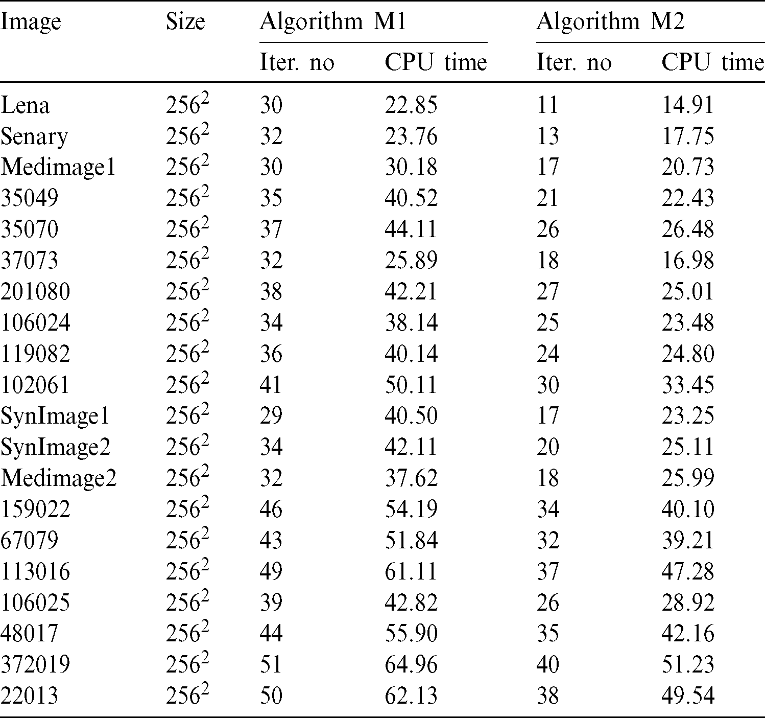
Test problem 1: In this experiment, two natural “Lena,” “Scenery,” one medical image” “MedImage1,” and images from Berkeley Segmentation Data Set (BSD 500) are picked as test images contaminated with multiplicative noise (Gama noise) having noise levels L1 = 17, L1 = 15, L1 = 15, L1 = 20, L1 = 20, and L1 = 20, respectively to analyze the restoration results of the schemes M1 and M2. All images are recorded respectively in Figs. 2–7. In all Figures in this experiment, (a) and (b) are the true and degraded images while (c) and (d) illustrates the reconstructed images by the two algorithms M1 and M2, respectively. In all imaging tests, it can be seen that algorithm M2 results in a better outcome regarding the visual quality of image restoration compared with algorithm M1. It can be noticed that the image restoration quality and preservation of edges of M1 are good, but struggle with the minimization of the staircase effect which is an inherent drawback of the TV-based technique along with mesh-based scheme M1 applied for PDE solution connected with TV functional. Similarly, M1 also suffers from the initial assumption which is a key to good restoration results. These reconstructed images generated by M1 are shown in Figs. 2c–7c, respectively. On the other hand, the image restoration results produced by the meshless algorithm M2 concerning visual quality, reduction of staircase effect, and edges preservation are superior to image restoration quality by mesh-based algorithm M1 because of the meshfree features of MQ-RBF approximation utilized to the smooth solution of the PDE connected with TV functional. All the restoration results for M2 are provided respectively in Figs. 2d–7d. Furthermore, the PSNR and SSIM values of image denoising by two algorithms M1 and M2 for the real and medical images “Lena,” “Senary,” and “MedImage1” and BSD 500 images are listed in Tab. 2. Tab. 2 reveals that the PSNR, SSIM, and SNR values concerning the image restoration of algorithm M2 are larger than algorithm M1, which shows the best restoration performance of M2 over M1. It can also be likewise noticed from Tab. 3 that computation time (CPU) and iterative numbers required for convergence of scheme M2 are less than scheme M1 which show the expedited recovery performance of proposed meshless algorithm M2 against the mesh-based algorithm M1 due to the meshless utilization of the decreased dependence on a mesh or integration method associated with MQ-RBF for the solution of PDE. The shape parameter c plays a vital part in the meshless procedure M2 which can affect the image denoising performance. We can also also see that some additional results for image restoration, iterative number, and time required for convergence from the BSD 500 data set have been provided in Tabs. 2 and 3, respectively. Thus in this analysis, the best optimal value of shape parameter c is kept in the range . Moreover, we also set .

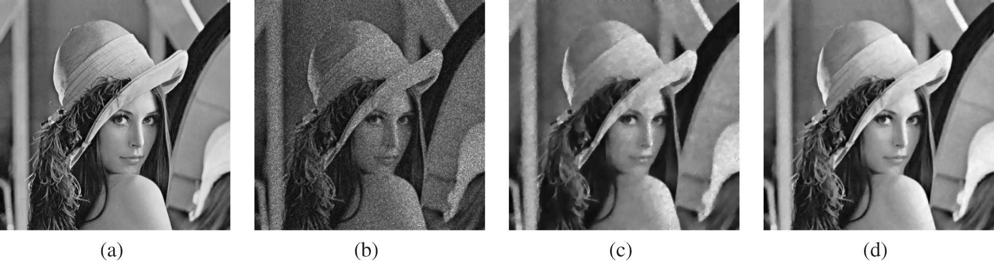
Figure 2: De-noised effects on Lena image. (a) Actual image. (b) Lena image contaminated with multiplicative noise L1 = 17. (c) Reestablished image using scheme M1. (d) Reestablished image using scheme M2 with c = 1.70, , and

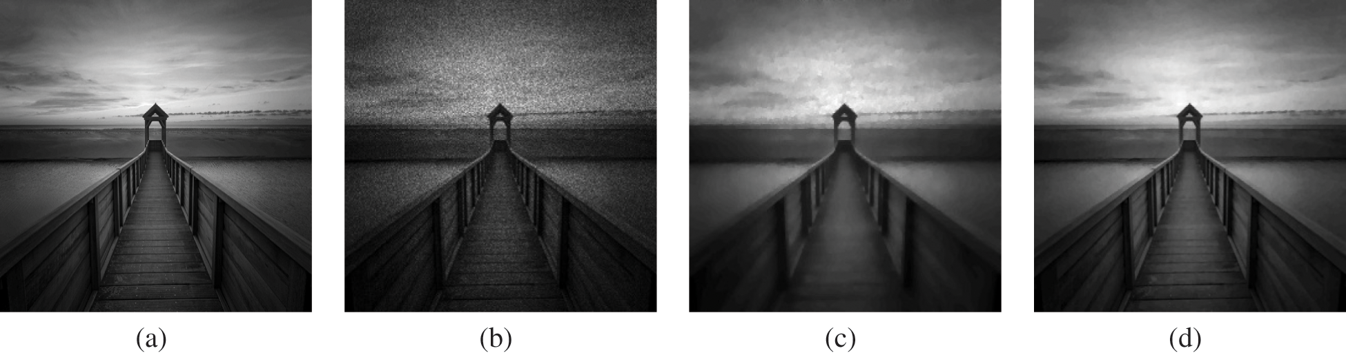
Figure 3: Achieved results on senary image. (a) Actual image. (b) Noisy image with multiplicative noise L1 = 15. (c) Obtained image using scheme M1. (d) Obtained image using scheme M2 with c = 1.66, , and

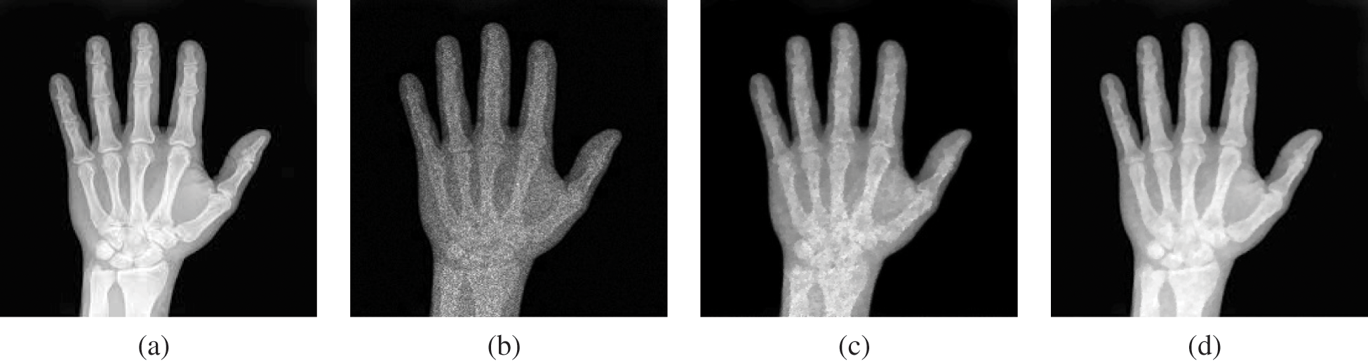
Figure 4: Produced results on medical image MedImage1. (a) Actual image. (b) Noisy image with multiplicative noise L1 = 15. (c) Improved image using scheme M1. (d) Improved image using scheme M2 with c = 1.74, , and

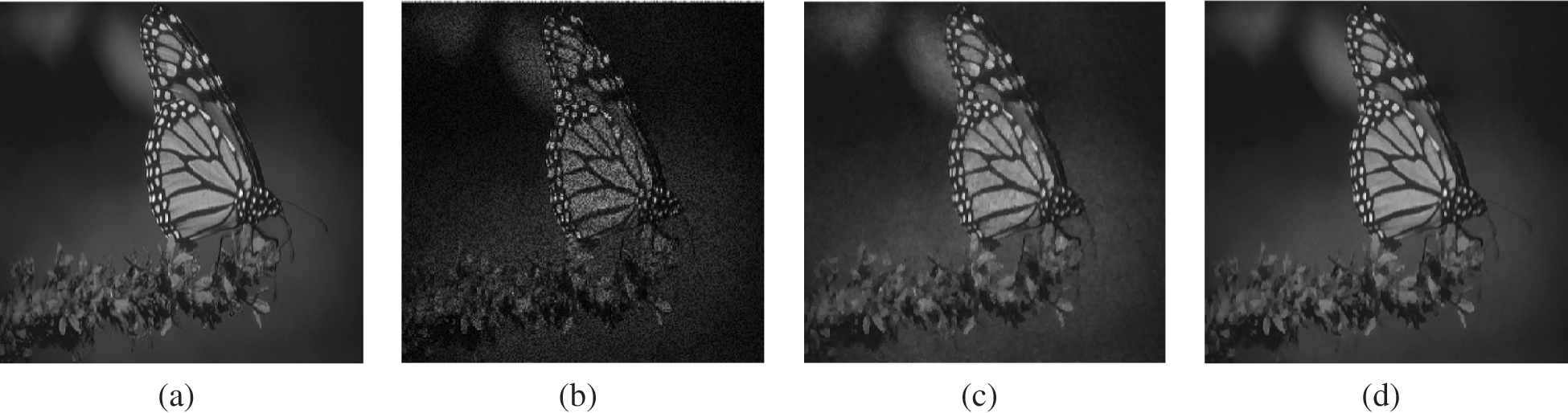
Figure 5: Developed outcomes on BSD (5000) image 35049. (a) Actual image. (b) Noisy image with multiplicative noise L1 = 20. (c) Rebuilt image using algorithm M1. (d) Rebuilt image using algorithm M2 with c = 1.73, 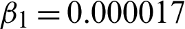, and

Figure 6: Reconstructed effects on BSD (5000) image 35070. (a) Actual image. (b) Noisy image with multiplicative noise L1 = 20. (c) Recorded image using algorithm M1. (d) Recorded image using algorithm M2 with c = 1.72, = 0.000015, and

Figure 7: Obtained effects on BSD (5000) image 37073. (a) Actual image. (b) Noisy image with multiplicative noise L1 = 20. (c) Reestablished image using scheme M1. (d) Reestablished image using scheme M2 with c = 1.72, , and

Table 2: PSNR, SSIM, and SNR values comparison of schemes M1 and M2

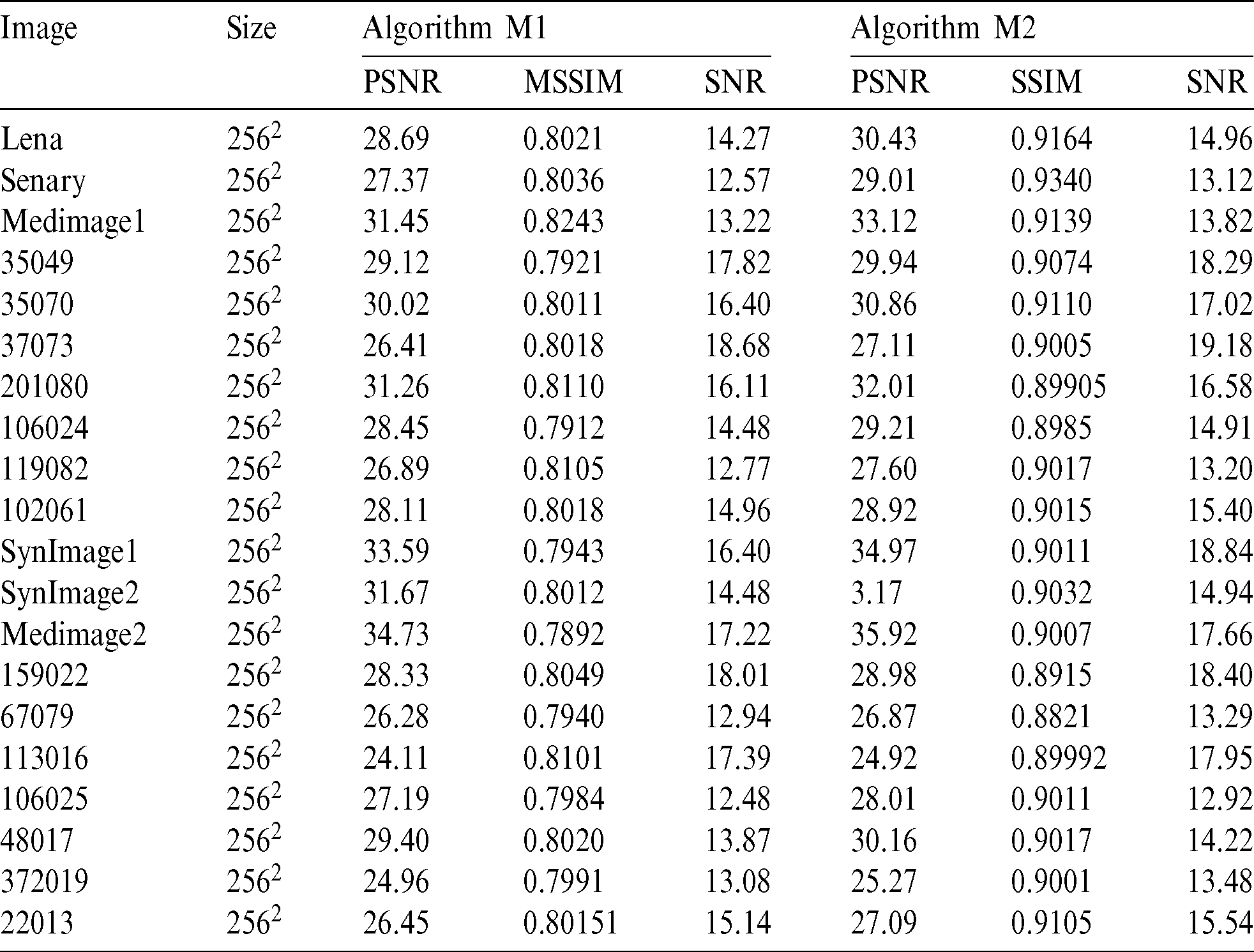
Table 3: Results of schemes M1 and M2 concerning the iterative numbers and CPU times (sec) needed for convergence

Test problem 2: In this experiment, the proposed meshless method M2 is investigated on artificial and medical images “SynImage1,” “SynImage2,” “MedImage2” and BSD 500 images which are shown respectively in Figs. 8–13. The noise levels chosen for all the images “SynImage1,” “SynImage2,” and “MedImage2” and BSD 500 are L2 = 16, L2 = 16, L2 = 15, L2 = 20, L2 = 20, and L2 = 20, respectively. In all the cases, the efficiency of image reconstruction by M2 is well-restored than M1. Repeatedly, M1 generates better restoration results simultaneously with edges preservation but struggles with the elimination of the staircase effect because of TV regularization and mesh-based technique used in M1. All the generated images by M1 are presented respectively in Figs. 8c–13c. However, the proposed scheme M2 gives an improved image restoration performance regarding the visual quality of image restoration, edges preservation, and minimization of the staircase effect than M1 due to the meshless applicability of MQ-RBF approximations implemented in algorithm M2. All the resultant images produced by M2 are given in Figs 8d–13d, respectively. The preference of the two techniques M1 and M2 concerning image recovery (PSNR, SSIM, and SNR values), and CPU time of computation and the iterative numbers needed for convergence for all the “SynImage1,” “SynImage2,” “MedImage2,” and BSD 500 images can be noted from Tabs. 2 and 3. Again, Tabs. 2 and 3 display the superiority of M2 over M1 concerning image restoration and faster convergence performance. We can also notice that some additional results for image restoration, iterative number, and time required for convergence from the BSD 500 data set have been provided in Tabs. 2 and 3, respectively. Repeatedly, the optimum value of the shape parameter c required for image denoising is set to 1.78 1.85. Here, we choose .

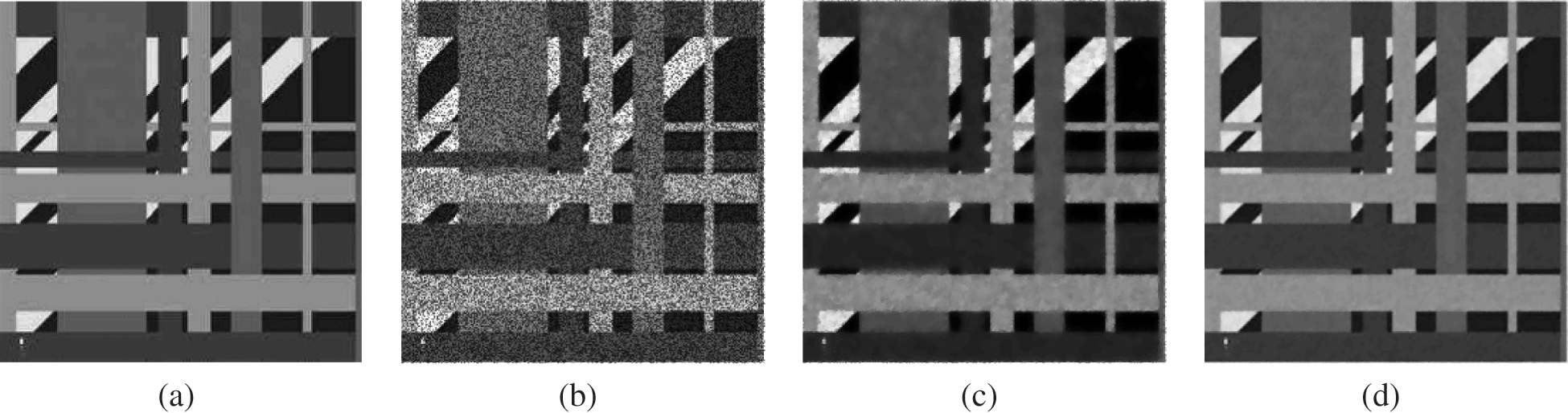
Figure 8: Reestablished effects on SynImage1 image. (a) Actual image. (b) Noisy image contaminated with speckle noise L2 = 16. (c) Obtained image using algorithm M1. (d) Obtained image using algorithm M2 with c = 1.84, , and

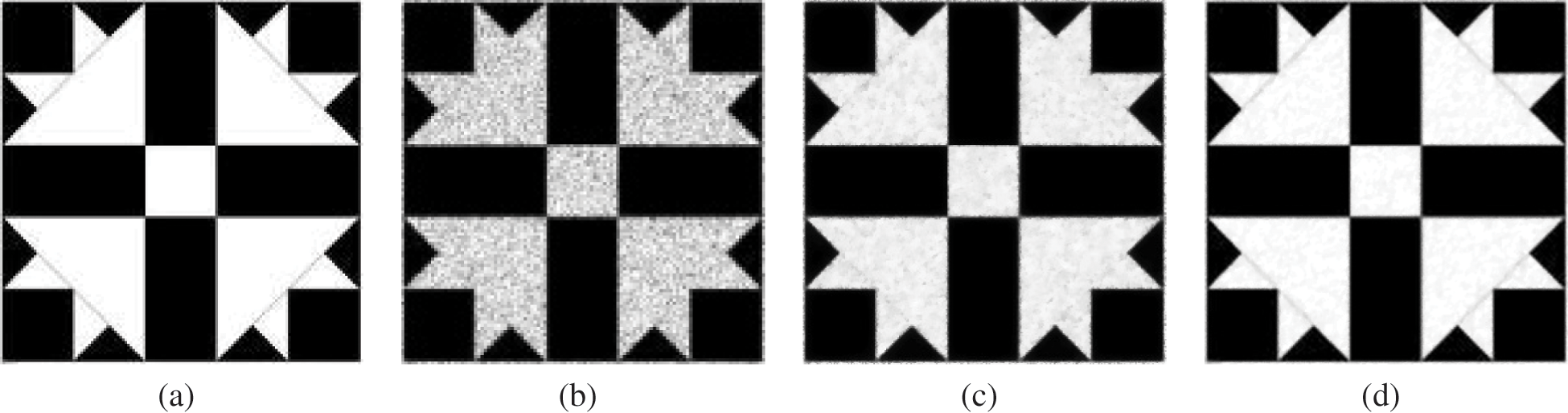
Figure 9: Test effects on SynImage2 image. (a) Actual image. (b) Degraded image with speckle noise L2 = 15. (c) Resultant image using method M1. (d) Resultant image using method M2 with c = 1.79, , and

Figure 10: Recovery resultant effects on medical image MedImage2. (a) Actual image. (b) MedImage2 image debased with speckle noise L2 = 16. (c) Rebuilt image using scheme M1. (d) Rebuilt image using scheme M2 with c = 1.80, , and

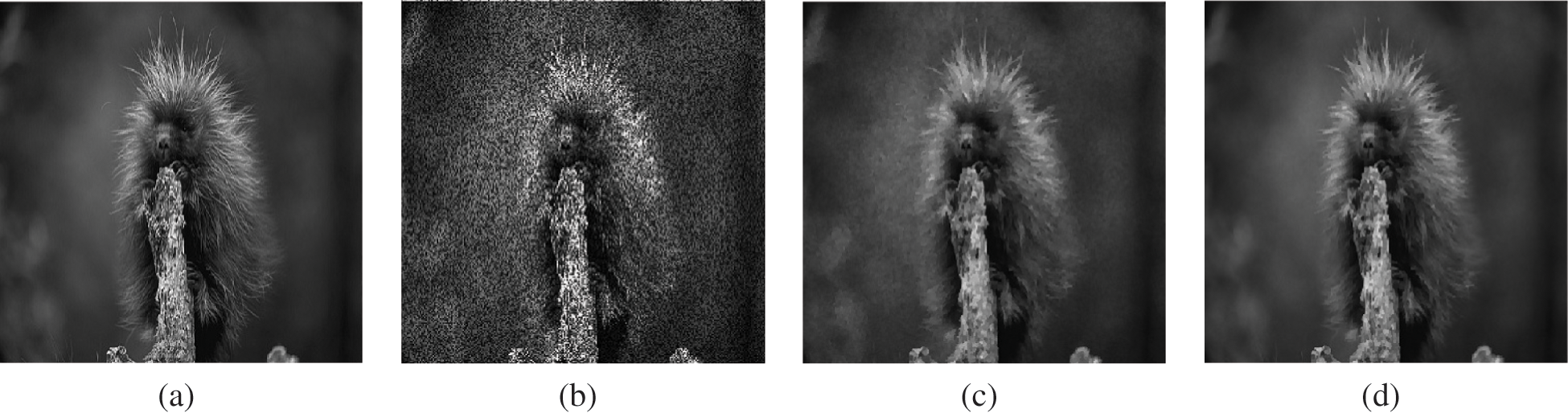
Figure 11: Recovered resultant effects on BSD (5000) image 159022. (a) Actual image. (b) BSD image corrupted with speckle noise L2 = 20. (c) Recovered image using scheme M1. (d) Recovered image using scheme M2 with c = 1.82, , and

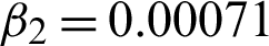
Figure 12: Obtained resultant effects BSD (5000) image 67079. (a) True image. (b) BSD image corrupted with speckle noise L2 = 20. (c) Denoised image using method M1. (d) Denoised image using method M2 with c = 1.83, , and

Figure 13: Recovered resultant effects on BSD (5000) image 159022. (a) True image. (b) BSD image corrupted with speckle noise L2 = 20. (c) Obtained image using scheme M1. (d) Obtained image using scheme M2 with c = 1.83, , and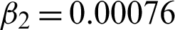

Test problem 3: In this investigation, the “Lena” image is picked for experimental results. Fig. 8 indicates a rectangular area of interest for the comparison of M1 and M2. In areas with edges, it is noticed that M2 recovers and improves the image characteristics in a more authentic approach than M1, which describes the more excellent achievement of edge improvement and reducing the staircase effect of M2 (appeared in zoomed-in Fig. 14d) over M1 (appeared in zoomed-in Fig. 14c) due to the meshless properties of MQ-RBF utilized in recommended scheme M2.

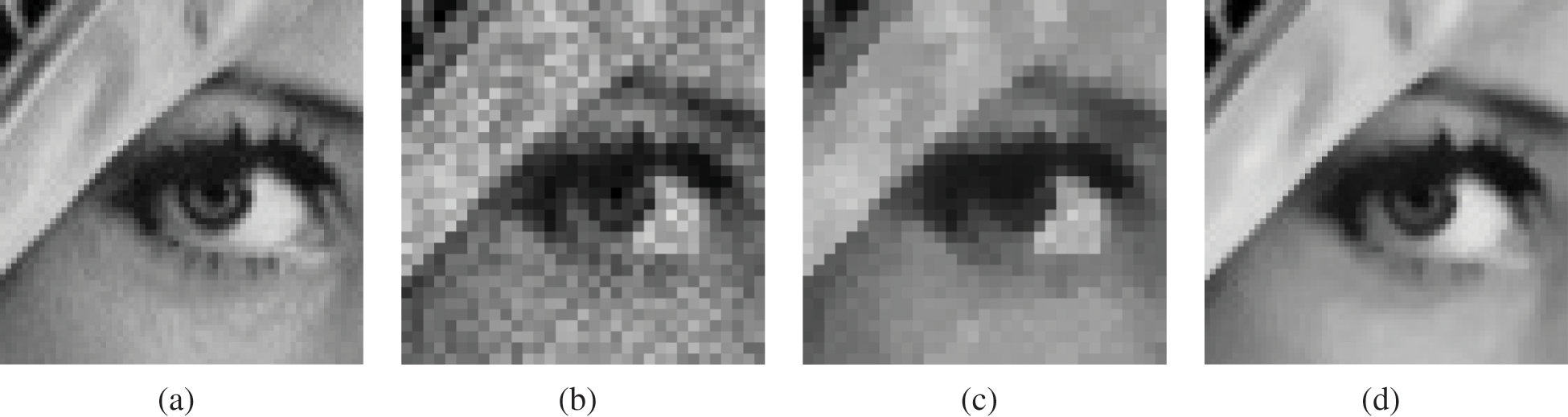
Figure 14: An area of “Lena” image with discontinuities. (a) Zoomed-in area of true image. (b) Zoomed-in area of noisy image. (c) Zoomed-in area obtained by method M1. (d) Zoomed-in area obtained with method M2

Test problem 4: In this analysis, the two schemes M1 and M2 are investigated for texture perseveration that has appeared in Fig. 15. It has been noticed from Fig. 15 that the textured areas are improved in a better way by using the M2 (shown in Fig. 15d) corresponded to M1 (shown in Fig. 15c) due to the meshless quality of MQ-RBF connected with algorithm M2.

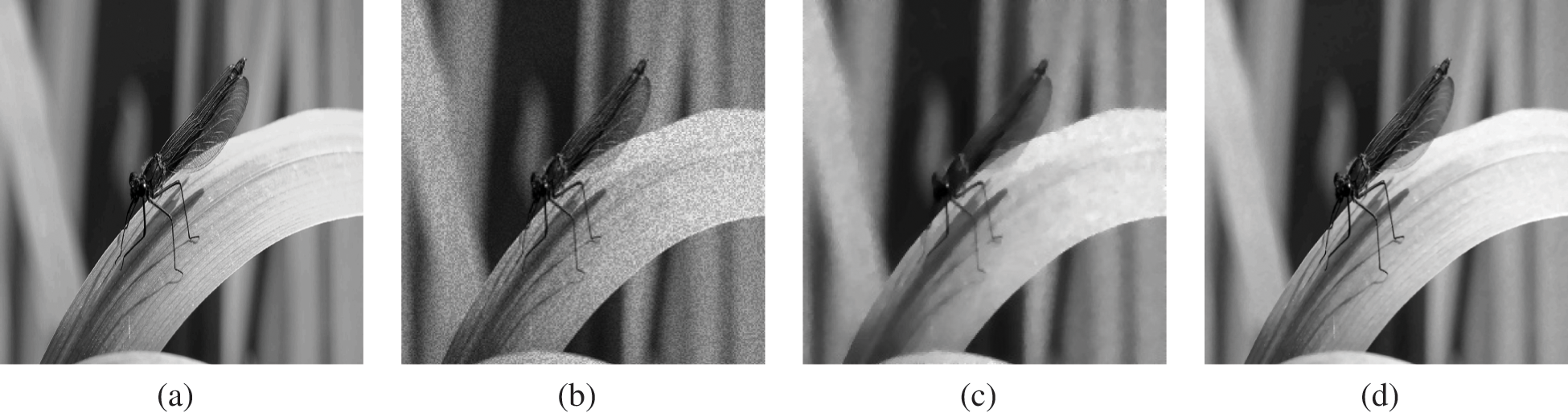
Figure 15: Experimental effects on synthetic texture image. (a) Actual image. (b) Noisy image. (c) Recovered result using scheme M1. (d) Recovered result using scheme M2

Test problem 5: In this test, the real image “Lena” is inquired to investigate the homogeneity and examine the loss (or preservation) for the two algorithms M1 and M2. For this investigation, different lines of true images are analyzed with noisy and denoised images which are presented in Figs. 16 and 17, respectively. We can notice that the reconstructed lines by meshless algorithm M2 (given in Figs. 16c and 17c) are superior to mesh-based algorithm M1 (given in the Figs. 16b and 17b) because of the meshfree utilization of MQ-RBF technique employed in algorithm M2.

Figure 16: The 199th line comparison of “Lena” image. (a) Actual and degraded images line comparison. (b) Actual and acquired image by algorithm M1 lines comparison. (c) Actual and acquired images by algorithm M2 lines comparison. The blue and red lines indicate the actual and reconstructed images

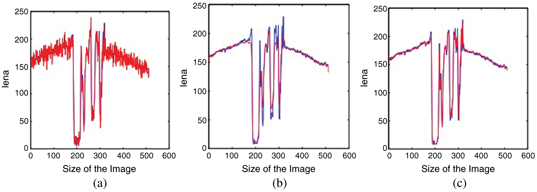
Figure 17: The 129th line comparison of “Lena” image. (a) Actual and degraded images line comparison. (b) Actual and acquired image by algorithm M1 lines comparison. (c) Actual and acquired images by algorithm M2 lines comparison. The blue and red lines indicate the actual and reconstructed images

5.1 Shape Parameter Analysis

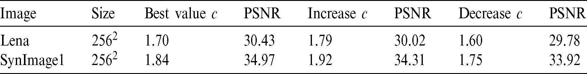
The shape parameter c performs an influential role in image restoration in meshless algorithm M2 which can influence the image reconstruction quality (PSNR). For this purpose, we choose different values of shape parameter c used in algorithm M2 for real and artificial images to examine the results on image restoration quality (PSNR). It can be seen from Figs. 18, 19, and Tab. 4 that various values of the shape parameter c influence the image recovery feature of real and artificial images “Lena” and “SynImage1.”

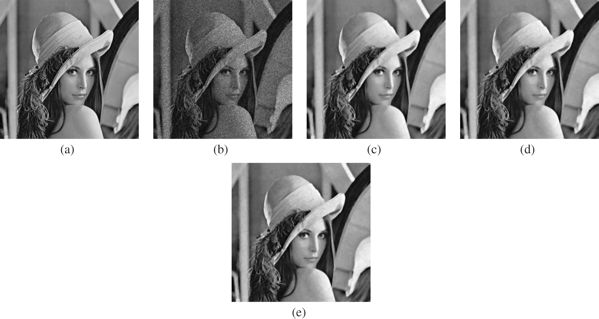
Figure 18: Experimental results on real image Lena. (a) True image. (b) Noisy Lena with multiplicative noise L1 = 17. (c) Obtained image using best selected value of c = 1.70. (d) Obtained image using c = 1.79. (e) Obtained image using c = 1.60

Figure 19: Test results on SynImage1. (a) True image. (b) Noisy SynImage1 image with multiplicative noise L2 = 16. (c) De-noised image using best selected value of c = 1.84. (d) De-noised image using c = 1.92. (e) De-noised image using c = 1.75

5.2 Comparison with Other Schemes

5.2.1 Comparison with Other Total Variation (TV) Schemes

In this subsection, the suggested meshless scheme M2 is compared to some TV-based methods used for multiplicative noise removal problems.

ROL Technique The ROL model is presented in [62], and its solution is also discussed and demonstrated in [62], which is presented by the resulting gradient projection iterative technique:

The experimental values of the two Lagrange multipliers , , and time step dt are already examined and described in [62].

AA Technique AA model is discussed and explained in [52] and its solution is done by the given gradient projection technique:

The most useful values for and dt are taken in the ROL method and Lagrange multiplier is discussed in [52].

HMW Technique The numerical solution HMW-model is presented in [22] (HMW-model is similar to SO-model when ). HMW-model is written as:

which leads to the following minimization algorithms;

The associated Euler–Lagrange equation of z is

The solution of z and w by Newton and Chambolle projection algorithms are already explained in [22]. The rules for terminating principle and the determination of the two regularization parameters and for this model are further discussed and suggested in [22].

In our computational experiments, we practice u(0) = f as the initial guess for ROL and AA models and for HMW model.

Table 4: Effects on image reconstruction concerning RSNR values of various values of shape parameter c practiced in meshless scheme M2 for real and artificial images

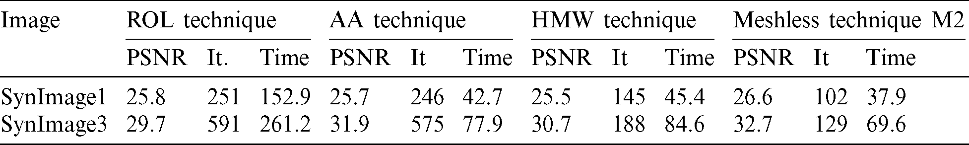
Test problem 5: The demonstrated results in Figs. 20, 21, and Tab. 5 suggest that the proposed algorithm M2 provides superior performance over ROL, AA and HMW approaches concerning the image restoration (PSNR), iterative numbers and CPU times required for convergence for the same images including same sizes and noise levels accompanying by the same parameters values of ROL, AA and HMW methods applied in [18] particularly when the noise variance is high. In this test the value of dt is selected as 0.07.

Figure 20: Resultant effects on SynImage1. (a) Actual image. (b) Noisy image by speckle noise L2 = 2. (c) Rebuilt image using technique RLO. (d) Rebuilt image using technique AA. (e) RRebuilt image using technique HMW. (f) Rebuilt image using proposed technique M2 with 1.90, , and

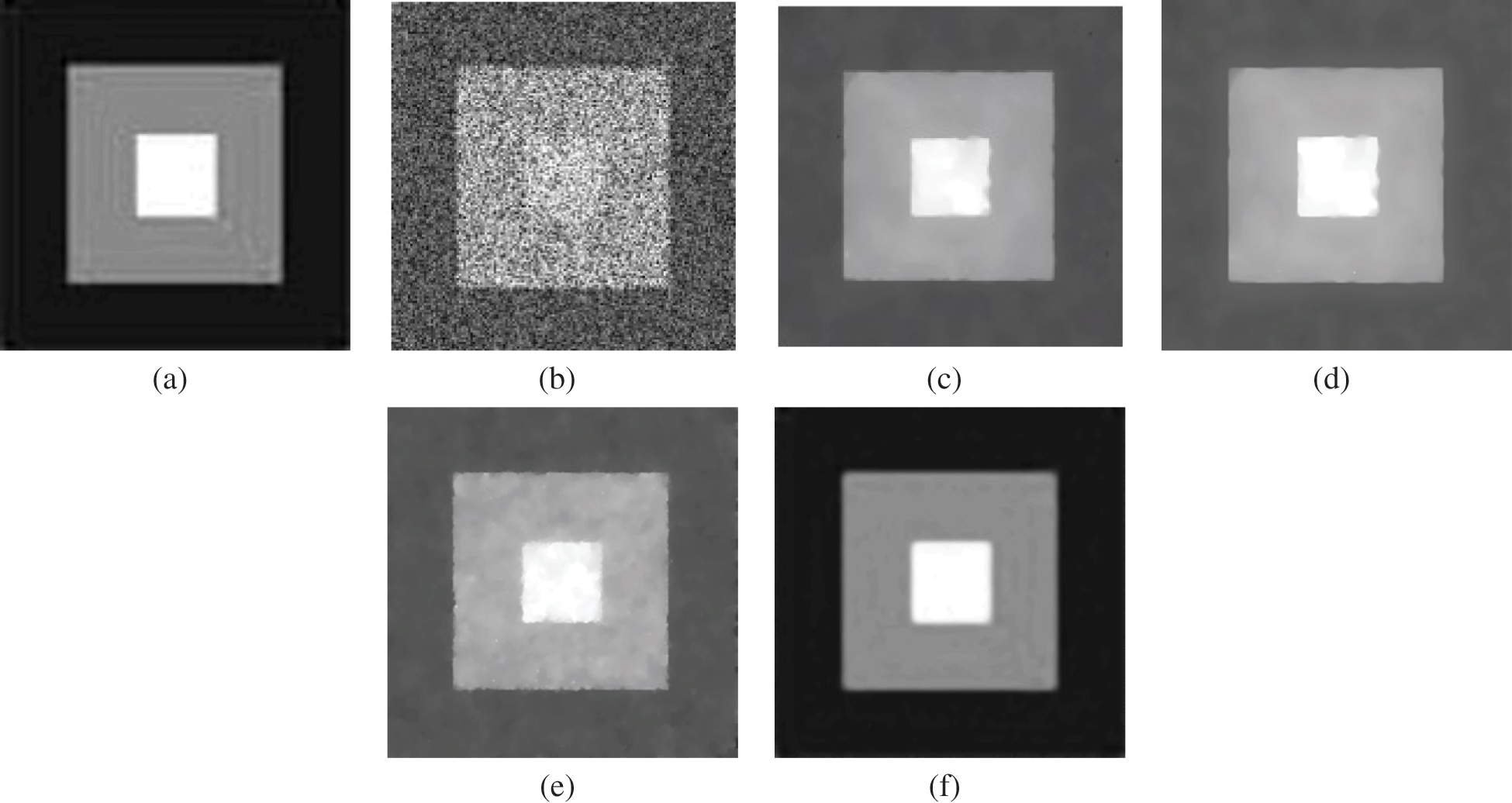
Figure 21: Rebuilt effects on SynImage3. (a) Actual image. (b) Noisy image connected with speckle noise L2 = 5. (c) Reassembled image using RLO scheme. (d) Reassembled image using AA scheme. (e) Reassembled image using HMW scheme. (f) Reassembled image using proposed meshless scheme M2 with c = 1.88, 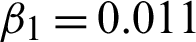, and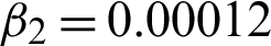

5.2.2 Multiplicative Noise Removal Using Primal-Dual and Reweighted Alternating Minimization (M3)

The author Wang et al. [63] has developed a new primal-dual iterative scheme to solve the PED equation connected with the minimization functional of the reweighed TV-based model. The mathematical model for this functional is given as:

with 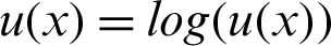and . Where is the regularization parameter in the functional (55), while g(x) shows the non negative weight function and mathematically expressed as follow.

where n and indicates the total number of outer iterations and stability of the iterations, respectively. The primal-dual iterative scheme splits the Eq. (55) for solution as recommended in [63] and is defined as below.

where w and are called the auxiliary function and regularization parameter, respectively. The regularization parameters shows the connection between w and u. The alternating minimization scheme is applied to divide Eq. (57) into two sub-equations which are given as follows.

Table 5: Comparison of models ROL, AA, HMW and proposed our method M2 regarding PSNR values, iterative numbers and CPU (time in sec) of the two artificial images of size 2562

where the first step to apply a weighted TV-based scheme to Eq. (58) for denoising to the step in which the image has multiplicative noise while the second Eq. (59) is used as the second step to solve the part of optimization. The primal-dual scheme is then utilized by the authors to define a convex closed set K as

in which represents the closed set of {.}. So by the above procedure, Eq. (55) is defend as follows.

The authors used the same procedure as done in (59) and defend another system of nonlinear of equation for Eq. (58) as

For more information about the primal-dual method, the readers are referred to [63].

Test problem 6: The judgment of the two algorithms M2 and M3 concerning the visual quality of image restoration (SNR) connected with two artificial and real images “SynImage4” and “Lena” are shown in Figs. 22 and 23 and recorded in Tab. 6 for the same image size, noise level, and parameter values as selected for M3 in [63]. It can be observed from Figs. 22 and 23 and Tab. 6 that the proposed algorithm M2 produces more reliable restoration performance regarding image restoration (SNR) and reducing the staircase effect from the two artificial and real images “SynImage4” and “Lena.” The value of dt is decided as 0.001.

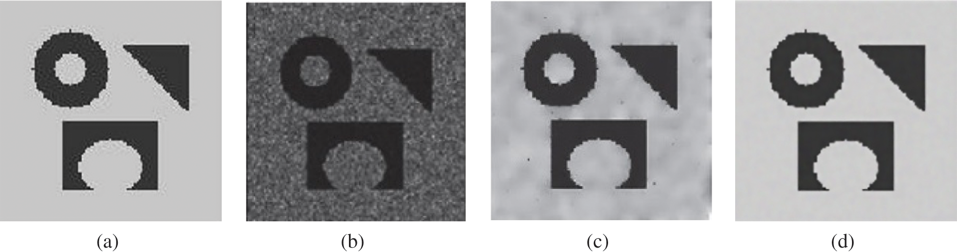
Figure 22: Experiential effects on artificial image SynImage4. (a) Actual image. (b) Noisy image with multiplicative noise with standard variance . (c) Reconstructed image using scheme M3. (d) Reconstructed image using scheme M2 with c = 1.77, 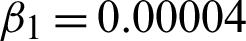, and

Figure 23: Test effects on Lena image. (a) Actual image. (b) Noisy image contaminated with standard variation . (c) Resultant image using procedure M3. (d) Obtained image using proposed procedure M2 with c = 1.74, , and

Table 6: SNR values of two algorithms M2 and M3 for comparison

6  Sensitivity Analysis of Parameters

This section is committed to the study of the choice of parameters utilized in algorithm M2. The three parameters i.e., c and fitting parameters and used in algorithm M2 are more difficult to determine. Nevertheless, their best-chosen values are fixed and then set according to the size and noise variance of the image. It has been seen the limit of the permitted values is: [1.65, 1.85], [0.00000924, 0.015], and [data-refids=0.00020, 0.009] for natural, artificial, and medical images according to the noise variation L1 = 17, 15, 15 and L2 = 16, 15, 16, respectively. These ranges acknowledge that the choice of the parameters c, , and are more important for the quality image restoration. Therefore, the selection of parameters is surprisingly important to avoid wrong decisions concerning image restoration. For uniformity, the subsequent information is done for Tabs. 7 and 8.

Table 7: Table for the percentage increase in the most suitable chosen values used in recommended method M2 and its corresponding percentage effect on the PSNR value of denoised image “Lena” of size 2562

Table 8: Table for the percentage decrease in the most suitable chosen values used in recommended method M2 and its corresponding percentage effect on the PSNR value of denoised image “Lena” of size 2562

1. ()% increase-, and ()% decrease-

2. For instance (0.20) stands for 0.20% decrease in PSNR

3. (0.77) stands for 0.77% increase in PSNR

7  Conclusion

In this research study, the Multiquadric radial basis function-based meshless collocation scheme was introduced for the numerical solution of nonlinear PDE connected with TV-based functional used for image restoration holding multiplicative noise. The presented methodology has experimented on different real, medical, and artificial images regarding multiplicative and speckle noises, and the results were compared to current TV-based traditional methods.

The numerical results have confirmed that restoration performance regarding the restoration quality (PSNR, SNR, and MSSIM values), minimization of staircase effect, preservation of edges and textures, and convergence process of the proposed scheme were more accurate and efficient than other schemes.

Nevertheless, the proposed meshless scheme yields an unsymmetrical interpolation matrix and lower accuracy in boundary-adjacent regions when the image size becomes very large. These issues are under construction and results will be stated in the succeeding paper.

Funding Statement: The author(s) received no specific funding for this study.

Conflicts of Interest: The authors declare that they have no conflicts of interest to report regarding the present study.

References

 1.  Aubert, G., Kornprobst, P. (2002). Mathematical problems in image processing. Applied Mathematical Sciences, 147(2), 149–309. [Google Scholar]

 2.  Chen, T. F., Shen, J. H. (2005). Image processing and analysis. E-publishing, SIAM: Philadelphia. pp. 1–97. [Google Scholar]

 3.  Dougherty, G. (2009). Digital image processing for medical applications, 1st edition. pp. 1–447. New York, USA: Cambridge University Press. DOI 10.1017/CBO9780511609657. [Google Scholar] [CrossRef]

 4.  Bao, P., Zhang, L. (2003). Noise reduction for magnetic resonance images via adaptive multiscale products thresholding. IEEE Transactions on Medical Imaging, 22(9), 1089–1099. DOI 10.1109/TMI.2003.816958. [Google Scholar] [CrossRef]

 5.  Donoho, D. L., Johnstone, M. (1995). Adapting to unknown smoothness via wavelet shrinkage. Journal of the American Statistical Association, 90(432), 1200–1224. DOI 10.1080/01621459.1995.10476626. [Google Scholar] [CrossRef]

 6.  Geman, S., Geman, D. (1984). Stochastic relaxation, gibbs distributions, and the Bayesian restoration of images. IEEE Transactions on Pattern Analysis and Machine Intelligence, 6(6), 721–741. DOI 10.1109/TPAMI.1984.4767596. [Google Scholar] [CrossRef]

 7.  Goldstein, T., Osher, S. (2009). The split Bregman method for L1-regularized problems. SIAM Journal on Imaging Sciences, 2(2), 323–343. DOI 10.1137/080725891. [Google Scholar] [CrossRef]

 8.  Jiang, D. H., Tan, X., Liang, Y. Q., Fang, S. (2015). A new nonlocal variational bi-regularized image restoration model via split Bregman method. EURASIP Journal on Image and Video Processing, 15(1), 1–10. [Google Scholar]

 9.  Khan, M. A., Chen, W., Ullah, A., Fu, Z. (2017). A mesh-free algorithm for ROF model. EURASIP Journal on Advances in Signal Processing, 1(53), 1–16.

10. Liu, X., Huang, L. (2014). A new nonlocal total variation regularization algorithm for image denoising. Mathematics and Computers in Simulation, 97(1), 224–233. DOI 10.1016/j.matcom.2013.10.001. [Google Scholar] [CrossRef]

11. Liu, X., Huang, L. (2014). An efficient algorithm for adaptive total variation based image decomposition and restoration. International Journal of Applied Mathematics and Computer Science, 24(2), 405–415. DOI 10.2478/amcs-2014-0031. [Google Scholar] [CrossRef]

12. Achim, A., Bezerianos, A., Tsakalides, P. (2001). Novel Bayesian multiscale method for speckle removal in medical ultrasound images. IEEE Transactions on Medical Imaging, 20(8), 772–783. DOI 10.1109/42.938245. [Google Scholar] [CrossRef]

13. Bratsolis, E., Sigelle, M. (2003). Fast SAR image restoration, segmentation, and detection of high-reflectance regions. IEEE Transactions on Geoscience and Remote Sensing, 41(2), 2890–2899. DOI 10.1109/TGRS.2003.817222.

14. Malladi, R., Sethian, J. A. (1996). A unified approach to noise removal, image enhancement, and shape recovery. IEEE Transactions on Image Processing, 5(11), 1554–1568. DOI 10.1109/83.541425.

15. Sheng, C., Xin, Y., Liping, Y., Kun, S. (2005). Total variation-based speckle reduction using multi-grid algorithm for ultrasound images. ICIAP, 3617, 245–252.

16. Steidl, G., Teuber, T. (2010). Removing multiplicative noise by Douglas–Rachford splitting methods. Journal of Mathematical Imaging and Vision, 36(2), 168–184. DOI 10.1007/s10851-009-0179-5.

17. Thanh, L. T., Thanh, D. N. H. (2019). Medical images denoising method based on total variation regularization and anscombe transform. 19th International Symposium on Communications and Information Technologies, pp. 26–30. Ho Chi Minh, Vietnam. [Google Scholar]

18. Huang, L. L., Xiao, L., Huiwei, Z. (2010). Multiplicative noise removal via a novel variational model. EURASIP Journal on Image and Video Processing, 5, 987–995. [Google Scholar]

19. Kansa, E. J. (1999). Motivation for using radial basis functions to solve PDEs. USA: Lawrence Livermore National Library. [Google Scholar]

20. Le, T., Vese, L. (2003). Additive and multiplicative piecewise-smooth segmentation models in a variational level set approach. In: UCLA CAM Report 03-52. Los Angeles, CA: University of California at Los Angeles. [Google Scholar]

21. Chen, D. Q., Cheng, L. Z. (2012). Spatially adapted total variation model to remove multiplicative noise. IEEE Transactions on Image Processing, 21(4), 1650–1662. DOI 10.1109/TIP.2011.2172801. [Google Scholar] [CrossRef]

22. Huang, Y. M., Ng, M. K., Wen, Y. W. (2009). A new total variation method for multiplicative noise removal. SIAM Journal on Imaging Sciences, 2(1), 22–40. DOI 10.1137/080712593. [Google Scholar] [CrossRef]

23. Krissian, K., Vosburgh, K., Kikinis, R., Westin, C. F. (2004). Anisotropic diffusion of ultrasound constrained by speckle noise model. Technical report. IEEE Computer Society Conference on Computer Vision and Pattern Recognition, vol. 2, pp. 547–552. San Diego, CA, USA.

24. Khan, M. A., Chen, W., Ullah, A., Ji, L. (2018). Euler’s elastica and curvature based model for image restoration. PLoS One, 13(9), 353–370. DOI 10.1371/journal.pone.0202464.

25. Ogier, A., Hellier, P. (2004). A modified total variation denoising method in the context of 3D ultrasound images. MICCAI, 3216, 70–77.

26. Rudin, L., Lions, P. L., Osher, S. (2003). Multiplicative denoising and deblurring: Theory and algorithms. vol. 3, pp. 103–119. New York, USA: Springer.

27. Shi, J., Osher, S. (2008). A nonlinear inverse scale space method for a convex multiplicative noise model. SIAM Journal on Imaging Sciences, 1(3), 294–321. DOI 10.1137/070689954.

28. Ullah, A., Chen, W., Khan, M. A. (2016). A new variational approach for restoring images with multiplicative noise. Computers & Mathematics with Applications, 71(10), 2034–2050. DOI 10.1016/j.camwa.2016.03.024. [Google Scholar] [CrossRef]

29. Rudin, L. I., Osher, S., Fatemi, E. (1992). Nonlinear total variation based noise removal algorithms. Physica D, 60(1–4), 259–268. [Google Scholar]

30. Rudin, L., Osher, S. (2003). Total variation based image restoration with free local constraints. IEEE Transactions on Image Processing, 1, 21–40.

31. Shen, J. (2003). Weber’ law and weberized TV restoration. Physica D, 175(3–4), 241–251. DOI 10.1016/S0167-2789(02)00734-0. [Google Scholar] [CrossRef]

32. Fasshauer, G. E. (1997). Solving partial differential equations by collections with radial basis functions. Proceedings of Chamonix, pp. 1–8. Nashville, USA. [Google Scholar]

33. Buhmann, M., Dyn, N. (1993). Spectral convergence of multiquadric interpolation. Proceedings of the Edinburgh Mathematical Society, 36(2), 319–333. DOI 10.1017/S0013091500018411. [Google Scholar] [CrossRef]

34. Sarra, S. A. (2009). Multiquadric radial basis function approximation methods for the numerical solution of partial differential equations. Artical, Marshall University and Edward J. Kansa University of California, USA. [Google Scholar]

35. Zerroukat, M., Power, H., Chen, C. S. (1998). A numerical method for heat transfer problem using collocation and radial basis functions. International Journal for Numerical Methods in Engineering, 42, 1263–1278. [Google Scholar]

36. Larsson, E., Fornberg, B. (2003). On the efficiency and exponential convergence of multiquadric collocation method compared with finite element method. Engineering Analysis with Boundary Elements, 27, 251–257. [Google Scholar]

37. Li, J., Hon, Y. C. (1983). Domain decomposition for radial basis meshless method. IEEE Transactions on Communications, 31(3), 388–397. DOI 10.1109/TCOM.1983.1095832. [Google Scholar] [CrossRef]

38. Larsson, E., Fornberg, B. (2003). A numerical study of some radial basis function based solution methods for elliptic PDEs. Computers & Mathematics with Applications, 46(5–6), 891–902. DOI 10.1016/S0898-1221(03)90151-9. [Google Scholar] [CrossRef]

39. Bernal, F., Gutirrez, G. (2009). Solving delay differential equations through RBF collocation. AAMM, 1(2), 257–272. [Google Scholar]

40. Chen, Y., Gottlieb, S., Heryudono, A., Narayan, A. (2016). A reduced radial basis function method for partial differential equations on irregular domains. Journal of Scientific Computing, 66(1), 67–90. DOI 10.1007/s10915-015-0013-8.

41. Dehghan, M., Abbaszadeh, M., Mohebbi, A. (2015). A meshless technique based on the local radial basis functions collocation method for solving parabolic–parabolic Patlak–Keller–Segel chemotaxis model. Engineering Analysis with Boundary Elements, 56, 129–144. DOI 10.1016/j.enganabound.2015.02.005.

42. Islam, S. U., Singh, V., Rajput, S. (2017). Estimation of dispersion in an open channel from an elevated source using an upwind local meshless method. International Journal of Computational Methods, 14(1), 1–14.

43. Islam, S. U., Sarler, B., Vertnik, R. (2013). Local radial basis function collocation method along with explicit time stepping for hyperbolic partial differential equations. Applied Numerical Mathematics, 67, 136–151. DOI 10.1016/j.apnum.2011.08.009. [Google Scholar] [CrossRef]

44. Driscoll, T. A., Fornberg, B. (2002). Interpolation in the limit of increasingly at radial basis functions. Computers and Maths & Applics., 43(3–5), 413–422. [Google Scholar]

45. Micchelli, C. A. (1986). Interpolation of scattered data: Distance matrices and conditionally positive definite functions. Constructive Approximation, 2(1), 11–12. DOI 10.1007/BF01893414. [Google Scholar] [CrossRef]

46. Sarra, S. A. (2006). Digital total variation filtering as postprocessing for radial basis function approximation methods. Computers and Maths & Applics., 52, 1119–11130. [Google Scholar]

47. Kansa, E. J. (1990). Multiquadrics–-A scattered data approximation scheme with applications to computational fluid dynamics I: Solutions to parabolic, hyperbolic, and elliptic partial differential equations. Computers and Maths & Applics., 19, 147–161. [Google Scholar]

48. Kansa, E. J. (1990). Multiquadrics–-A scattered data approximation scheme with applications to computational fluid dynamics II: Surface approximations and partial derivative estimates. Computers and Maths & Applics., 19, 127–145. [Google Scholar]

49. Liu, K. (2016). Radial basis functions: Biomedical applications and parallelization. (Thesis and Dissertations). Ke Liu University of Wisconsin-Milwaukee, USA. [Google Scholar]

50. Sajavičius, S. (2013). Optimization, conditioning and accuracy of radial basis function method for partial differential equations with nonlocal boundary conditions. Engineering Analysis with Boundary Elements, 37(4), 788–804. DOI 10.1016/j.enganabound.2013.01.009. [Google Scholar] [CrossRef]

51. Savage, J. D. (2006). Fast iterative methods for solving large systems arising from variational models in image processing, (Ph.D. Thesis). University of Liverpool, UK. [Google Scholar]

52. Aubert, G., Aujol, J. F. (2008). A variational approach to removing multiplicative noise. SIAM Journal on Applied Mathematics, 68(4), 925–946. DOI 10.1137/060671814. [Google Scholar] [CrossRef]

53. Buhmann, M. (2003). Radial basis functions: Theory and implementations, 1st edition. UK: Cambridge University Press. [Google Scholar]

54. Chen, W., Fu, Z. J., Chen, C. S. (2014). Recent advances in radial basis function collocation, 1st edition. Germany: Springer. [Google Scholar]

55. Schaback, R. (2007). A practical guide to radial basis functions. Numerical Algorithm, 45, 345–368. [Google Scholar]

56. Wright, G. B. (2008). Radial basis function interpolation: Numerical and analytical developments (Ph.D. Thesis). University of Colorado, Boulder. [Google Scholar]

57. Dyn, N. (1989). Interpolation and approximation by radial and related function. vol. 1, pp. 211–234. UK: Cambridge University Press. [Google Scholar]

58. Vogel, C. R., Oman, M. E. (1996). Iterative methods for total variation denoising. SIAM Journal on Scientific Computing, 17(1), 227–238. DOI 10.1137/0917016. [Google Scholar] [CrossRef]

59. Trefethen, L. N., Ban III., D. (1997). Numerical linear algebra. SIAM, 50, 1–361. [Google Scholar]

60. Madych, W. R., Nelson, S. A. (1990). Multivariate interpolation and conditionally positive definite functions II. Mathematics of Computation, 54(189), 211–230. DOI 10.1090/S0025-5718-1990-0993931-7. [Google Scholar] [CrossRef]

61. Thanh, D. N. H., Hai, N. H., Prasath, V. B. S., Hieu, L. M., Tavares, J. M. R. S. (2020). A two-stage filter for high density salt and pepper denoising. Multimedia Tools and Applications, 79(29–30), 21013–21035. DOI 10.1007/s11042-020-08887-6. [Google Scholar] [CrossRef]

62. Rudin, L. I., Lions, P. L., Osher, S. (2003). Multiplicative denoising and deblurring: Theory and algorithms. In: Geometric Level Set Methods in Imaging, Vision, and Graphics, pp. 103–120. Berlin, Germany: Springer. [Google Scholar]

63. Wang, X., Bi, Y., Feng, X., Huo, L. (2016). Multiplicative noise removal using primal-dual and reweighted alternating minimization. SpringerPlus, 5(1), 925. DOI 10.1186/s40064-016-1807-3. [Google Scholar] [CrossRef]

Appendix:

The derivatives utilized in the proposed meshless scheme M2 in Eq. (42) are defined as follows:

By recalling Eq. (33) which is given as under:

To find the derivative using N evaluation data points () and Nc data center points (), then by RBF interpolation we get the given equation.

or

which results in () evaluation matrix D, i.e.,

Next, the first derivative from (64) displays as

or

where

By the combination of Eqs. (63) and (68) results in the given differential equation.

Define S = DC −1, then above Eq. (70) is re-written as

where the differentiation matrix is written by the following equation.

Similarly, the second order derivative is also mathematically given as under.

Likewise

As it is acknowledged that the matrix C is invertible, so the differentiation matrix is well-defined.

For any adequately differentiable RBF, [r(x)], then by applying chain rule, we obtain the resulting derivatives.

for the first derivative accompanying with

The second order derivative is calculated by the given equation.

with

For any the basis function, in particular Multiquadric (MQ), we have

and

This work is licensed under a Creative Commons Attribution 4.0 International License, which permits unrestricted use, distribution, and reproduction in any medium, provided the original work is properly cited.